Identifiability of stiffness from isotope-resolved Raman shifts asks which stiffness parameters become determined once the moving masses are independently constrained. In the assigned harmonic oscillator model of reduced-mass ambiguity in a Raman stiffness inference,Here $c$ is the speed of light, ${\tilde{\nu }}_i$ the vibrational wavenumber and ${\mu }_i$ the mode's known effective mass. Known masses and identified modes make each effective stiffness identifiable within this model. Unknown masses still permit the simultaneous rescaling $(k_i,{\mu }_i)\mapsto (a{k}_i,a{\mu }_i)$ without changing a frequency; knowing only mass ratios determines only stiffness ratios.

Controlled isotope substitution is useful because it changes nuclear mass while approximately preserving the interatomic force model. In a pure-carbon mode for which every moving mass changes by the same ratio, unchanged stiffness predictsThe mass numbers here are an explicit approximation. They replace a full normal mode calculation only for the stipulated uniform mass scaling.

For an original numerical test, a chosen carbon-12 reference band at $1580\mathrm{c}{\mathrm{m}}^{-1}$ predicts about $1518.01\mathrm{c}{\mathrm{m}}^{-1}$ after uniform carbon-13 replacement with unchanged stiffness. If a hypothetical carbon-13 band is instead $1520\mathrm{c}{\mathrm{m}}^{-1}$, its isotope-corrected Raman stiffness ratio isThe residual inferred change is about $0.262\%$, not the several-percent softening one would infer by ignoring mass. This is a chosen calculation, not a quoted experimental peak pair.

The primary graphene study measured several Raman bands at different carbon-13 concentrations and laser excitation energies; its measured mass-dependent frequencies followed the harmonic-oscillator relation.^[ref] Such a controlled series tests the mass model. It does not by itself rule out changes in strain, temperature or mode mixing in a different sample. Uncertainty in isotope composition, spectral calibration and mode assignment must accompany any small residual stiffness inference.

The mean cumulative postoperative event count is the expected number of specified postoperative episodes accumulated per operated patient by a stated time. It measures repeated event burden, rather than only whether a patient had any event. An event definition must distinguish a new episode from continued observation of an existing complication.

Let $N_i(t)$ be patient $i$'s counting process for qualifying events up to postoperative time $t$. The population target isWith complete observation of $n$ independent patients through $t$, its empirical estimate isThis can exceed one. In contrast, the probability of at least one event is $p(t)=\mathrm{Pr}(N_i(t)\ge 1)$ and cannot exceed one. The inequality $\mu (t)\ge p(t)$ follows because each patient with any event contributes at least one to the count.

For an original five-patient example, counts $(0,0,0,0,5)$ give $\hat{\mu }=1$ and an observed any-event fraction $1/5$. Counts $(1,1,1,1,1)$ also give mean count $1$, but any-event fraction $1$. The same mean burden can describe very different distributions across patients. Neither count summary encodes the severity of each episode.

Uncertainty should respect the patient as the sampling unit. At fixed $t$, write $K_i=N_i(t)$ and calculateThe first example has $s_K^2=5$ and estimated standard error $1$. Treating its five events as five unrelated patient outcomes would discard the observed clustering. A small-sample estimated standard error is not itself a validated confidence interval.

Death and incomplete follow-up require explicit definitions. For accumulated burden per original operated patient, events cease at death but events already experienced remain counted; the denominator is not silently restricted to survivors. D. Ghosh and D. Y. Lin studied the marginal mean cumulative number of recurrent events in the presence of a terminal event, including nonparametric estimation and comparison.^[ref]

Loss to follow-up hides later events, whereas death prevents them. Simply averaging the available patients at each time can change the target population. Suitable observation-process assumptions and a censoring-aware method are needed for incomplete data. Comparisons should also show mortality: fewer accumulated events can accompany shorter survival, rather than reduced morbidity among otherwise comparable survivors.

Branch selection by a controlled beam-radius change resolves which of the reciprocal radius ratios is present in a centred Gaussian heterodyne overlap measurement. In reciprocal size-ratio ambiguity in centred Gaussian overlap, the efficiency is $\eta (\rho )=4{\rho }^2/(1+{\rho }^2{)}^2$, with $\rho =w_2/w_1$. Its local signed response isAn infinitesimal increase of the second radius therefore improves overlap when $\rho <1$ and worsens it when $\rho >1$, provided curvature, displacement and polarization stay fixed.

A finite one-sided change needs more care. For a known multiplier $q>1$, direct comparison givesThe threshold is below one because the finite change can overshoot the optimum. In an original example, $\rho =0.99$ is initially on the narrower-beam branch, with efficiency about $0.99990$. Increasing that radius by $10\%$ gives $\rho =1.089$ and efficiency about $0.9928$. The observed decrease alone would misclassify the initial branch if interpreted using the infinitesimal rule.

Use a symmetric beam-radius perturbation for overlap branch selection when two controlled settings are available. Compare $\eta (q\rho )$ with $\eta (\rho /q)$. Since the efficiency is an even, strictly decreasing function of $|\log \rho |$, their difference is positive for $\rho <1$, negative for $\rho >1$, and zero at matching. In the same example with $q=1.10$, the two efficiencies are about $0.9928$ and $0.9890$, correctly selecting the initially narrower beam. The perturbation must be large enough to resolve above measurement noise.

NIST's physical heterodyne setup used beam combination, polarization control and single-mode collection to establish optical matching.^[ref] A practical radius change must preserve those other mode properties; an arbitrary lens adjustment can change wavefront curvature as well and invalidate this one-variable diagnostic.

The group delay introduced by a capacitive amplifier load is the negative angular frequency derivative of the extra wave phase produced by that load. For the resistive output model in reactive-load phase shift in a finite-output-impedance amplifier, divide the loaded transfer function by the unloaded one:The added group delay is thereforeThis subtraction of unloaded wave phase prevents the amplifier's intrinsic group delay from being attributed to the capacitor. The terminal model uses a Thévenin equivalent; the group delay definition differentiates an unwrapped wave phase, as in the SciPy signal-processing documentation. Its digital-filter function reports samples, whereas the analog derivative above uses radians per second and gives seconds.^[ref][ref]

For an original example, choose $R=200\Omega$ and $C=10\mathrm{nF}$, hence $\tau =2\mu \mathrm{s}$. At $\omega \tau =1$, corresponding to $f=1/(2\pi \tau )\approx 79.6\mathrm{kHz}$, the added group delay is $1\mu \mathrm{s}$. The same operating point has $-{\varphi }_{\mathrm{rel}}/\omega =\pi \tau /4\approx 1.571\mu \mathrm{s}$: a single sinusoid's phase displacement and the delay of a narrow frequency packet need not agree.

A practical test applies a weakly modulated carrier, varies its central frequency, and measures the output modulation displacement while comparing loaded and unloaded operation. The group delay describes that narrow-band envelope only when the frequency response varies slowly across its bandwidth. The corresponding causal impulse response begins at zero time, $h(t)=e^{-t/\tau }/\tau$ for $t\ge 0$, and vanishes for $t<0$; it is not a rigidly translated impulse. Thus group delay versus pulse-front arrival for an RC load matters when a measured pulse is broad enough to change shape.

The shot-noise precision of a Raman gain ratio is the statistical precision expected from finite detected photoelectron numbers under a stated counting model. Write the Raman pump-on pump-off gain ratio as $G=AD/(BC)$, where $A,B$ are pump-on probe/reference counts and $C,D$ pump-off probe/reference counts. For large independent Poisson counts, applying first-order propagation to $\log G$ givesThe parent article derives the equal-count limit. Independence, large counts and a calibrated conversion from readout units to photoelectrons are assumptions, not consequences of taking a ratio.

An original imbalanced example has ${\mu }_A={\mu }_B={\mu }_C=10^6$ and ${\mu }_D=10^4$. The relative standard uncertainty is about $\sqrt{0.000103}=1.015\%$. Increasing the three bright channels tenfold only reduces it to about $1.0015\%$: the weakest count channel dominates. Multiplicative detector-gain corrections can make the mean ratio appropriate to the optical experiment, but they do not create additional photoelectrons.

A simple photon-budget allocation for a Raman gain ratio makes the trade-off explicit. If the four mean counts sum to $N_{\mathrm{tot}}$, the Cauchy-Schwarz inequality givesEquality in this ideal unconstrained budget requires equal counts. Near unity gain, four approximately equal means totalling $4\times 10^6$ give about $0.2\%$ relative precision. Actual optical ratios, reference splitting and exposure constraints may prevent exact equality.

The primary FSRS experiment explicitly compared its computed photoelectron shot-noise limit with observed baseline noise and found additional detector structure; it averaged repeated gain spectra and discussed pixel-dependent corrections.^[ref] A counting limit is therefore a useful benchmark, not a guarantee of achieved experimental sensitivity.

Raman peak-fit uncertainty characterizes the uncertainty of a spectral-band position estimated by fitting a model to a Raman spectrum. It accompanies a Raman peak-position map: a colour difference between pixels need not establish a physical shift if the estimated positions are insufficiently precise. In Raman mapping, the instrument collects spectra at successive sample positions, and fitting extracts band parameters such as position and width.^[ref]

For an isolated band, a least squares fit might estimate the center, height, width and background of a Gaussian function. The uncertainty assigned to its center is conditional on the chosen model and description of spectral noise. Repeating the complete acquisition and fit at one unchanged location provides another assessment: if $n$ independent center estimates have standard deviation $s$, the estimated standard uncertainty of their sample mean is $s/\sqrt{n}$. This reduction applies to independent variation; it does not eliminate an offset shared by every acquisition.^[ref]

For an original numerical example, model two fitted positions aswhere $c$ represents a shared uncertain additive correction from measurement calibration, while $e_0,e_1$ are independent fitting errors, also independent of $c$. Suppose their standard uncertainties are $u(c)=0.10\mathrm{c}{\mathrm{m}}^{-1}$ and $u(e_i)=0.05\mathrm{c}{\mathrm{m}}^{-1}$. Each position then has combined standard uncertainty $\sqrt{0.10^2+0.05^2}\approx 0.112\mathrm{c}{\mathrm{m}}^{-1}$. Their difference cancels the same $c$, givingHere $u$ denotes standard uncertainty, so the difference has uncertainty about $0.0707\mathrm{c}{\mathrm{m}}^{-1}$. The covariance term is essential: treating the two positions as entirely independent would instead give about $0.158\mathrm{c}{\mathrm{m}}^{-1}$. A common additive correction cancels only insofar as it really is shared; instrument drift between measurements or a scale error need not cancel.^[ref]

For a hypothetical stress model $\sigma =({\hat{\nu }}_1-{\hat{\nu }}_0)/K$ with an exactly known illustrative $K=2\mathrm{c}{\mathrm{m}}^{-1}/GPa$, this difference uncertainty contributes $0.0354\mathrm{GPa}$ to the standard uncertainty of stress. Uncertainty in $K$ would require its own contribution. Raman peak-model bias, overlapping bands, an inadequate background and laser-induced sample changes can invalidate an otherwise small fit error. Retaining spectra and repeating fits with physically defensible models therefore matters alongside quoting a numerical uncertainty.

Raman integration-window bias is a systematic difference between the spectral-band area one intends to compare and the area captured by a selected finite Raman shift interval. It can create contrast in a Raman band-area map when the complete band area is unchanged: shifting or broadening redistributes intensity across the fixed interval's edges. The target must be stated clearly, because an area over that interval can be correctly measured even when it is a biased proxy for the complete band.

For an original calculation, take an isolated background-corrected Gaussian function bandIts complete area is $A_{\mathrm{full}}=Hs\sqrt{2\pi }$. Integrating only from $a$ to $b$ gives the Raman captured-area fractionwhere $\Phi$ is the cumulative distribution function of the standard normal distribution. The substitution $z=(\tilde{\nu }-{\tilde{\nu }}_0)/s$ gives this expression directly. The complete area depends on height and width; the captured fraction also depends on center position relative to the window.

Suppose $s=2\mathrm{c}{\mathrm{m}}^{-1}$ and the fixed window runs from996 to1004cm⁻¹. A center at1000cm⁻¹ places its edges at two standard widths on each side, giving $f=\Phi (2)-\Phi (-2)\approx 0.95450$. Shift the center to1004cm⁻¹ without changing height or width: now $f=\Phi (0)-\Phi (-4)\approx 0.49997$. The measured fixed-window area falls to about52.38% of its previous value although the complete band area is identical. This contrast is therefore insufficient evidence for a decrease in the amount of material.

A window that follows the fitted center can keep the captured fraction constant for this ideal fixed-width model. Broadening, neighboring bands, errors in a Raman peak-position map and an imperfect background still matter; a larger window can admit unwanted signal. Manufacturer documentation explicitly distinguishes simple intensity images from fitted-band analysis and warns that broad background can contaminate intensity contrast.^[ref] Reporting the actual interval, background treatment and whether the interval moves with the band makes the Raman band-area map scientifically interpretable.

A pulse-energy interval from incomplete tail measurements combines measured energy with bounds on optical power outside the acquisition window. It describes a set of compatible total energies, not automatically a standard uncertainty or confidence interval. The pulse-energy bounds from tail duration and pedestal height article treats a particular peak-and-width model; a window-based construction need not assume that pulse shape.

Suppose true radiant energy inside a measured window $G$ lies in a justified interval $[L,H]$, with $0\le L\le H$. Partition the unobserved times into regions of durations ${\Delta }_j$ with independently established nonnegative radiant power caps $M_j$. ThenFor an original measurement, let the observed-window energy lie between $48$ and $52\mathrm{nJ}$. An unobserved early region lasting $2\mathrm{ns}$ at most $0.50\mathrm{W}$ contributes at most $1\mathrm{nJ}$; a late region lasting $20\mathrm{ns}$ at most $0.20\mathrm{W}$ contributes at most $4\mathrm{nJ}$. The total interval is therefore $48$ to $57\mathrm{nJ}$. For these assumptions the fraction of optical energy outside a time gate equal to $G$ is at most $5/(48+5)\approx 9.43\%$.

A finite support cutoff is sufficient but not necessary for a finite bound. Bounding unobserved optical energy with an exponential tail model uses a validated cap $P(t)\le P_b{e}^{-(t-b)/\tau }$ after the window endpoint $b$, which integrates to $P_b\tau$. Without a justified duration or integrable envelope, one below-threshold reading cannot bound all later energy.

Establish the caps with characterized detector sensitivity, baseline and temporal coverage; do not identify detector ringing directly with optical tails. NIST's response analysis explicitly models the electrical trace as a convolution of the optical waveform with detector response.^[ref] The interval above follows from chosen optical bounds, not from an uncorrected finite-bandwidth detector trace.

Hydroxyproline denotes hydroxylated derivatives of proline, with an additional hydroxyl group on the ring. An important collagen-related form is Trans-4-hydroxy-L-proline. The substitution position and stereochemistry matter: a shared amino-acid framework does not specify every spatial arrangement.

In collagen biosynthesis, prolyl 4-hydroxylase modifies selected proline residues in a pre-existing polypeptide. Its reaction requires oxygen and 2-oxoglutarate, and its function depends on suitable iron and ascorbate availability. The resulting hydroxyproline residues support formation of the collagen triple helix.^[ref]

This is a post-translational modification: knowing the encoded sequence does not by itself establish that the chemical maturation step occurred. A structural comparison makes that measurable. Replacing a ring carbon's hydrogen with a hydroxyl group adds one oxygen atom overall, increasing the molecular mass by approximately $16\mathrm{Da}$ per site. Ten such modifications would add approximately $160\mathrm{Da}$ to a chain. These are stoichiometric expectations, not experimental measurements.

A mass change can support an assignment, but position and configuration require additional evidence. An observed increase of the right size alone does not identify which residue was modified or establish that the mature protein has formed its expected structure.

The displacement power factor is $\cos {\phi }_1$, where ${\phi }_1$ is the phase difference between the fundamental components of terminal electric potential difference and electric current. It describes phase displacement at that frequency. For purely sinusoidal signals it equals total power factor; with distorted waveforms those quantities can differ. The one-frequency phase relation follows from the RMS average-power expression.^[ref]

For a purely sinusoidal potential difference of RMS magnitude $V$ and zero-mean periodic current, orthogonality of harmonics givesThe ratio $I_1/I_{\mathrm{rms}}$ is the current distortion factor under these assumptions. A displacement factor near one does not establish that the whole current waveform closely follows the supply sinusoid.

For an original example, let the supply be100V RMS. Let the fundamental current be4A RMS at a lagging phase with cosine0.8, and add a3A RMS third harmonic. Total RMS current is5A, active power320W and apparent power500VA. The displacement factor is0.8 while total power factor is0.64.

Now cancel only the fundamental quadrature current, whose magnitude is $4\sqrt{1-0.8^2}=2.4\mathrm{A}$. The remaining in-phase fundamental is3.2A and the third harmonic is still3A. RMS source current is $\sqrt{3.2^2+3^2}\approx 4.39\mathrm{A}$, so total factor is about0.73 even though the displacement factor has become one. This illustrates a limitation of phase-only power factor correction, not a universal model of a correcting device.

The cosine also loses lead/lag sign: phases $+{\phi }_1$ and $-{\phi }_1$ have the same displacement factor but opposite sinusoidal reactive power. Retain the phase or lead/lag convention when that distinction matters. If the potential difference itself contains harmonics, total active power needs the contributions of the corresponding harmonic pairs; this simple fundamental-only reduction is no longer sufficient.

Power factor correction changes the current drawn from a source so that a specified active power is supplied with a more favorable power factor. For a sinusoidal inductive load, a parallel capacitor can supply an opposite reactive power component. It changes the source current's quadrature component while an ideal lossless correction branch leaves the load's active power unchanged.

Let the original load absorb $P+j{Q}_L$ at RMS potential difference $V$ and angular frequency $\omega$. A parallel ideal capacitance contributes $Q_C=-\omega C{V}^2$, soTo change a lagging phase angle from ${\phi }_1$ to a smaller lagging angle ${\phi }_2$ at fixed $P>0$,These follow from complex electrical power and the capacitive phase relationship.^[ref]

For an original ideal example, take $P=1000\mathrm{W}$, $V=200\mathrm{V}$ and50Hz. An initial factor0.8 corresponds to750var. A target factor0.95 corresponds to about328.68var, so a capacitance about33.53µF supplies the difference. RMS source current changes from6.25A to about5.26A. Resistive feeder loss at fixed resistance changes by $(0.8/0.95{)}^2\approx 0.709$, while the1000W load conversion remains the same in this model.

Reactive power overcompensation occurs if the capacitive contribution exceeds the intended inductive component. The net $Q$ then changes sign; continuing to add capacitance does not keep improving the magnitude of the factor. At a different load or frequency the same component can produce another result. Component ratings and nonideal circuit behavior require their own model rather than being determined by this one-frequency algebra.

Correction of displacement power factor is also distinct from correction of waveform distortion. Harmonic current can remain after the fundamental quadrature component is canceled. A useful measurement compares synchronized source potential-difference/current waveforms, RMS magnitudes and their average product before and after a change, retaining the operating condition. Separately measuring only RMS magnitudes cannot establish the resulting active power.

The current distortion factor is the ratio $D_I=I_1/I_{\mathrm{rms}}$, where $I_1$ is the root mean square magnitude of the fundamental electric current component and $I_{\mathrm{rms}}>0$ is the root mean square magnitude of the complete electric current. Its square is the fraction of the current's mean square supplied by the fundamental component. This ratio is distinct from displacement power factor, which measures the relative phase of the fundamental potential difference and current.

Use a Fourier series at fundamental frequency $\omega /(2\pi )$:Here $I_0$ is the DC component and the $I_n$ are RMS magnitudes of harmonic components. Averaging over a complete period, orthogonality and the Parseval identity giveFor purely sinusoidal electric potential difference $v(t)=\sqrt{2}V\cos \omega t$, only the fundamental electric current contributes to active power:Thus a displacement power factor of one can coexist with a lower total power factor.

For $I_1>0$, use fundamental-normalized current total harmonic distortion, ${\mathrm{THD}}_I=\sqrt{{\sum }_{n\ge 2}{I}_n^2}/I_1$. The relation between current distortion factor and THD with DC current isWith zero DC component, this reduces to $D_I=(1+{\mathrm{THD}}_I^2{)}^{-1/2}$. The definition of RMS here includes the DC component. For example, a 10 ampere fundamental and 3 ampere DC component, with no higher harmonic components, have zero total harmonic distortion but $D_I=10/\sqrt{109}\approx 0.9578$.

For an original zero-mean waveform, take a 230 volt RMS sinusoidal supply, $I_1=10\mathrm{A}$, $\cos {\varphi }_1=0.8$, and RMS third/fifth harmonic components of 6 and 3 amperes. ThenThe active power is 1840 watts, apparent power is about 2769.57 volt-amperes and total power factor is about 0.6644. This is an illustrative waveform model, not a measurement of a particular rectifier.

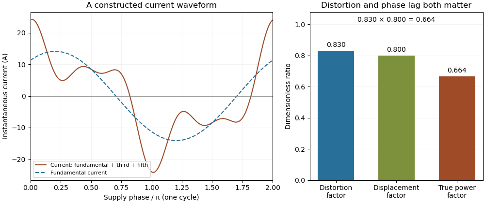
Terminology requires care. Overview of Functions: Harmonic Measurements by Schneider Electric uses distortion factor for the ratio of power factor to the fundamental cosine. Power Quality Considerations by Schneider Electric uses the label for harmonic content relative to the fundamental, or total harmonic distortion. The defining ratio identifies the intended quantity.

If the supply also contains harmonic components, use the harmonic active power sum:with matching voltage/current phase conventions. The fundamental-only factorization above assumes a purely sinusoidal supply.

A leading power factor describes an absorbing sinusoidal electrical load whose electric current leads its terminal electric potential difference. Under the passive sign convention, writeThe current maximum occurs earlier by $\theta /\omega$. The complex electrical power isThe negative reactive power is consistent with a capacitive terminal response. It does not imply negative mean absorbed active power.

For an original $100\mathrm{V}$, $2\mathrm{A}$ example with $\theta =\pi /3$, the power factor magnitude is $0.5$, active power is $100\mathrm{W}$, and reactive power is $-100\sqrt{3}\approx -173.21\mathrm{var}$. At $50\mathrm{Hz}$ the current leads by $1/(6f)\approx 3.33\mathrm{ms}$. A load with the same RMS magnitudes and the opposite phase displacement has identical active power but a lagging power factor and opposite reactive power.

For an ideal capacitor, $i=Cdv/dt$ gives a quarter-cycle current lead. Its mean active power is zero, although instantaneous power alternates as electrical energy enters and leaves the field. The primary one-frequency power derivation separates this quadrature exchange from net energy transfer.^[ref]

An inductive load can acquire a leading power factor at the source when power factor correction supplies more capacitive reactive power than the load absorbs. The current reduction interval for shunt reactive compensation shows why mildly leading operation can still draw less source electric current than no correction, while excessive correction reverses that benefit.

Record phase direction or signed reactive power together with the numerical factor. The same positive cosine can describe leading and lagging loads, and a meter may assign a separate sign according to its display convention.^[ref] For nonsinusoidal signals, state whether leading describes the fundamental displacement power factor; the complete power factor also depends on waveform distortion.

A lagging power factor describes an absorbing sinusoidal electrical load whose electric current lags its terminal electric potential difference. With the passive sign convention, chooseThe current maximum occurs later by $\phi /\omega$. The RMS phasors give complex electrical powerIn this equation the supply phasor is the real number $V$, while $I^{\ast }$ denotes the conjugate of the current phasor. Positive $Q$ is inductive reactive power under this convention. The primary MIT notes derive the conjugation and the peak-versus-RMS factor.^[ref]

For an original $230\mathrm{V}$, $10\mathrm{A}$ example with $\cos \phi =0.8$, active power is $1840\mathrm{W}$ and reactive power is $1380\mathrm{var}$. At $50\mathrm{Hz}$, $\phi \approx 0.6435$ radians corresponds to a current delay of about $2.05\mathrm{ms}$. The factor $0.8$ gives the magnitude of the phase relationship, while the word lagging supplies the direction lost by the cosine.

An ideal inductor is the limiting case $\phi =\pi /2$: it alternately stores and returns magnetic energy, with zero mean active power. An absorbing resistive-inductive load usually has both positive active power and positive reactive power. An ideal parallel capacitor can reduce the source's quadrature electric current; sufficient extra capacitance eventually crosses into leading power factor rather than improving the factor indefinitely.

For distorted waveforms, specify whether lagging refers to the fundamental displacement power factor; one phase angle does not characterize arbitrary harmonic components. A signed meter display is also not a universal lead/lag label. The manufacturer's sign-convention explanation distinguishes phase direction from the convention used for displayed factor signs.^[ref]

A principal polarization of an abelian variety $A$ is a polarization of an abelian variety $\lambda :A\to A^{\vee }$ that is an isomorphism. Equivalently, its isogeny has degree one. It identifies $A$ with its dual abelian variety through positivity supplied by an ample line bundle; an arbitrary isomorphism with the dual need not be a polarization of an abelian variety.^[ref]

For an elliptic curve $E$ with origin $0$, the degree-one line bundle ${\mathcal{O}}_E(0)$ gives a principal polarization. Replacing it by ${\mathcal{O}}_E(n\cdot 0)$, for positive $n$, multiplies the corresponding map to the dual by $n$ and gives degree $n^2$. Thus positivity alone does not make a polarization of an abelian variety principal: the size of its kernel matters.

A background-dependent photoresistor spectral response is the differential change of a photoresistor's output with wavelength-specific illumination, evaluated at a stated background state. It can depend on illumination level, spectral composition, bias, temperature and prior adaptation. The primary CdS datasheet specifies light-adaptation preconditioning before electrical tests, demonstrating that a measurement condition includes more than the instantaneous lux value.^[ref]

Let the steady electrical conductance be a functional $G=\mathcal{F}[E_{\lambda }]$ of incident spectral irradiance. About a background $E_{\lambda ,0}$, define the local response byThis derivative concerns small changes after specifying the operating state. A finite change or rapid modulation needs further nonlinear or dynamic characterization. Photoresistor spectral calibration establishes the required optical and electrical conditions.

An original separable model makes a useful distinction. Suppose $g=\int a(\lambda )E_{\lambda }(\lambda )d\lambda$ and $G=G_d+\kappa g^{\gamma }$, with positive $g,\kappa ,\gamma$. ThenThe amplitude changes with background, but the normalized spectral shape remains $a(\lambda )$. With $\gamma =0.7$, quadrupling $g_0$ multiplies the absolute differential response by $4^{-0.3}\approx 0.6598$. For a small one-percent generation increment, the leading fractional conductance change above the dark contribution is $0.7\%$; the exact model gives $(1.01{)}^{0.7}-1\approx 0.69895\%$.

A change in spectral shape requires more than that single separable nonlinearity. For an illustrative two-band response in dimensionless input coordinates, letThe derivatives are $\partial G/\partial E_a=1/(2\sqrt{E_a})$ and $\partial G/\partial E_b=1$. Changing the first-band background from $E_a=1$ to $4$ changes their ratio from $1/2$ to $1/4$. This toy model shows how relative spectral sensitivity can change; it is not measured behavior of a named component. Separable and nonseparable photoresistor spectral-response models should consequently be distinguished in a calibration analysis.

Resistance readout adds another operating-point factor: since $R=1/G$, $\delta R=-\delta G/G_0^2$. A resistance-divider output has yet another derivative. Comparing raw electrical slopes without converting to the same output variable can imitate a change in material response. Likewise, equal illuminance need not mean equal detector excitation, because the photopic luminous efficiency function supplies a different spectral weighting.^[ref]

A proposed apparatus combines a stable background source with a weak wavelength-selectable probe beam, a monitored reference detector and a fixed illumination geometry. At each background, measure the output derivative while decreasing probe amplitude to test the small-signal regime, then repeat after the prescribed settling or adaptation period. Normalize spectra only after retaining their absolute scale. This separates a changing overall gain from a changing spectral shape and from readout loading; it does not assume that a curve measured at one background transfers to every illumination condition.

The stress-optic law relates stress-induced birefringence to a mechanical stress difference. For an initially optically isotropic material in a suitable linear regime,where ${\sigma }_1,{\sigma }_2$ are the principal stresses normal to the light path and $C(\lambda )$ is the stress-optic coefficient. Its units are $\mathrm{P}{\mathrm{a}}^{-1}$, and its wavelength dependence matters when comparing optical measurements.^[ref]

For uniform thickness $t$ and uniform relevant stress directions along the path, the measured phase retardation isThe measurement determines a difference, not both stresses separately. States $(20,5)\mathrm{MPa}$ and $(40,25)\mathrm{MPa}$ have the same difference and therefore the same retardation in this model. Extra mechanical information is needed to separate their absolute stress components.

A uniaxial calibration specimen gives a practical coefficient measurement. With axial force $F$, known sectional area $A$ and negligible transverse stress, ${\sigma }_1-{\sigma }_2=F/A$. If retardation plotted against force has slope $s=d\delta /dF$, thenFor illustrative $s=0.003\mathrm{rad}{\mathrm{N}}^{-1}$, $\lambda =532\mathrm{nm}$, $A=20\mathrm{m}{\mathrm{m}}^2$ and $t=2\mathrm{mm}$, this gives $C\approx 2.54\times 10^{-12}\mathrm{P}{\mathrm{a}}^{-1}$. A $200\mathrm{N}$ load would give $10\mathrm{MPa}$ stress difference and $0.60$ radians retardation. These are chosen calibration numbers, not a universal coefficient for a plastic.

A polariscope with controlled loading, a force readout and polarization analysis supplies the relevant apparatus.^[ref] Background birefringence, thickness, temperature and wavelength should be accounted for. A measured intensity alone can have multiple compatible phase delays, and a changing optical-axis direction through a three-dimensional specimen can invalidate the simple scalar-path formula. The law is most useful when its optical and mechanical assumptions are checked together.

A photoconductor transient with quadratic recombination is a carrier-density model in which the loss rate grows as the square of the mobile excess density. It explains how nonlinear loss can produce different turn-on and turn-off waveforms without assigning unrelated exponential lifetimes to the two directions. A photoconductor converts illumination-dependent electrical conductivity into a signal under external bias; the manufacturer's primary PbS description establishes that conversion mechanism.^[ref] The quadratic loss law below is an explicitly stipulated model, not a fitted specification of that detector.

Assume a spatially uniform excess density $n\ge 0$, generation rate $g\ge 0$, constant coefficient $\beta >0$ and an output proportional to $n$ at fixed mobility and bias:Density has units ${\mathrm{m}}^{-3}$, $g$ has units ${\mathrm{m}}^{-3}{\mathrm{s}}^{-1}$ and $\beta$ has units ${\mathrm{m}}^3/s$. A two-carrier recombination rate proportional to the product of equal electron and hole densities motivates a quadratic term in an appropriate regime. Background carriers, other loss processes, contacts and trapping can invalidate that specialization.

For constant $g>0$, set $n_{\infty }=\sqrt{g/\beta }$ and $k=\beta n_{\infty }$. Separating variables, or differentiating the following expression, gives the solution for any finite nonnegative initial density $n_0$:For $n_0=0$ it reduces to $n_{\infty }\tanh (kt)$. For $n_0=n_{\infty }$ it stays at equilibrium, and for $n_0>n_{\infty }$ it approaches the same equilibrium from above. In the dark, $g=0$ instead yieldsThe reciprocal-density plot is linear in this model, while a semilogarithmic decay plot is curved. The dark half-decay time is $1/(\beta n_0)$, so it depends on the starting illumination.

The small-signal lifetime under quadratic recombination is different again. Linearize about a nonzero background $\overline{n}=\sqrt{\overline{g}/\beta }$:A locally exponential small-signal response can therefore coexist with a strongly nonexponential large dark transient. One measured time constant cannot be substituted for all three quantities.

For an original example, stipulate $\beta =10^{-15}{\mathrm{m}}^3/s$ and $\overline{n}=10^{18}{\mathrm{m}}^{-3}$. Then $\overline{g}=10^{21}{\mathrm{m}}^{-3}{\mathrm{s}}^{-1}$, dark half-decay time $1\mathrm{ms}$, small-signal lifetime $0.5\mathrm{ms}$ and small-signal half-power frequency about $318.3\mathrm{Hz}$. Four times the background generation doubles equilibrium density and doubles that frequency in this model.

A proposed test measures small modulation about several backgrounds separately from complete turn-off traces, while controlling actual detector bias, temperature and readout response. Examine reciprocal-density linearity only after justifying how the measured current maps to density. A successful fit supports the tested rate-law approximation; it does not uniquely identify the microscopic electron-hole recombination mechanism. Temperature and spectral sensitivity also vary in real PbS detectors and must be held or measured independently.^[ref]

An instability tongue is a tongue-shaped region in parameter space where a periodically forced linear system has an exponentially growing mode. In the Mathieu equationFloquet theory detects instability through a Floquet multiplier of modulus greater than one. The exactly zero solution remains zero, and initial data on a decaying mode need not grow.

Near the principal resonance $a=1$ with small $q$, multiple-scale analysis gives the leading growth rateIt is real and nonzero inside the leading region $|a-1|<|q|$. The exact boundary has corrections beyond this approximation. The width therefore opens from zero at the resonance point, giving the tongue shape.

Unlike additive resonance, the drive here changes a coefficient of the equation. Detuning $a-1$ competes with that parametric coupling; damping and nonlinear saturation can further change the instability region and long-time behavior.^[ref]