Topics (384k) Articles (398k) Users (410) Discussions (242) Comments (383) Files (13k) New article

Photon-budget allocation for a Raman gain ratio distributes measurement effort among the channels entering a ratio. For four large independent Poisson photoelectron counts with means , the shot-noise precision of a Raman gain ratio has approximate relative variance . With a freely allocatable fixed total expected count , the minimum is at equal counts. The constraint matters: fixed total exposure time is a different optimization problem.
Suppose channel has known photoelectron rate and an independently adjustable exposure . Estimate the optical ratios from exposure-normalized rates, so the known exposure factors are included. Then and a total time budget givesThe Cauchy-Schwarz inequality, or differentiation with a constraint multiplier, givesThis exposure-time allocation for a Raman gain ratio spends longer on weak channels without necessarily equalizing their final counts.
For an original one-second budget, let two rates be and two be photoelectrons per second. The optimal exposures are second for each bright channel and second for each weak channel. Expected counts are about and respectively, with relative standard uncertainty . Four equal exposures would give about instead. The gain comes from allocating the stated resource more efficiently, not creating additional information by normalizing counts.
The primary FSRS detector records probe and reference spectra together and alternates pump-on/off exposures.[ref]
Femtosecond Broadband Stimulated Raman: A New Approach for High-Performance Vibrational Spectroscopy by David W. McCamant and others. Data Collection, shutters, paired spectra, equation 4 and averaging
Such linked channels cannot have four independently chosen exposure times; the appropriate grouped constraints must replace the ideal model above. Read noise, dark uncertainty, saturation and sample change can alter the optimum as well.A self-complementary RNA duplex population describes how identical RNA strands are distributed between free strands and duplexes under specified conditions. A fraction of strands in duplexes differs from a fraction of molecular objects that are duplexes. The distinction matters when comparing chemical mass balances with observed signals.
For the ideal equilibrium , let and . With dimensionless association constant and reference molar concentration , define . The strand balance givesThis is the population model underlying ideal self-complementary RNA duplex melting. It assumes separated strands and duplexes are the only relevant species and that chemical equilibrium is reached.
The concentration regimes are illuminating. For , ; for , . An original calculation gives at and at . Even a large association parameter leaves some free strands in this equilibrium model.
An original finite-count illustration has 100 strands,80 of which belong to 40 duplexes, with 20 free strands left. The paired-strand fraction is 0.8, but duplexes are of the 60 molecular objects. A detector responding equally to each object would not give the same signal as a detector responding equally per strand. RNA optical melting needs a model of the folded and unfolded optical responses to infer populations.
Differentiating the equilibrium relation givesAt , a small 10% relative change in changes by approximately 0.0167. Population is therefore not generally proportional to concentration.
Competing RNA hairpins require an expanded species balance. A primary tetraloop study evaluated hairpin and duplex formation explicitly when designing sequences for melting experiments.[ref]
Thermodynamic characterization of naturally occurring RNA tetraloops by Justin P. Sheehy and others. Materials and Methods, Design of sequences for optical melting studies.
Ignoring a populated competitor can produce a precise solution to the wrong balance equation.RNA log-odds covariance describes correlated errors between transformed population estimates at different temperatures in an RNA melting log-odds plot. Shared RNA melting baselines can generate it even when individual detector readings are independent.
Let be unfolded fractions and . First-order propagation givesIn matrix form, with diagonal . This is the multivariate form of RNA melting log-odds uncertainty; the derivatives are evaluated at the estimated fractions.[ref]
A concrete shared-input model uses . If all folded-state predictions contain the same uncertain offset , thenThis component has one shared error direction. It is not equivalent to adding independent noise with variance to every observation. Other baseline parameters contribute through RNA baseline prediction covariance.
For an original simplified example, nine observations each have independent log-odds standard uncertainty0.03 and the same shared-offset contribution 0.01. The standard uncertainty of their mean isIncorrectly treating the shared term as independent would give . Repetition reduces the independent component while leaving this common offset contribution intact.
A model fit can use the joint covariance matrix in generalized least squares, with an objective of the form when that inverse exists. Alternatively, fit the underlying absorbance and baseline parameters jointly. Shared-error components alone may be singular, and near population endpoints the logarithmic linearization may fail. A precise straight-line fit does not independently validate the two-state RNA melting model or its baseline assumptions.
The variance of a pedestal-corrected sample quantifies the random spread remaining after subtracting an estimated baseline from a signal acquisition. Subtracting a mean reset charge-injection pedestal removes an offset; it does not automatically remove reset pedestal variance. For a raw signal sample and pedestal estimate ,The covariance term determines whether subtraction suppresses shared fluctuations or adds independent noise. The GUM's correlated-input rule gives this identity directly for the linear measurement model .[ref]
Two correction procedures have different statistical consequences. First suppose signal acquisitions have independent pedestals of variance and independent readout noise of variance . A separate mean of independent blank acquisitions, with individual variance , is reused for every signal sample:After removing any constant means, independence givesConsequently, averaging corrected samples givesThe shared blank correction creates a common uncertainty floor, as in shared calibration error.
Alternatively, a baseline and signal reading from the same acquisition can share a fluctuating pedestal. In an idealized correlated double sampling model, and , so : the common cancels. Independent readout noises remain and their variances add. More generally, if paired readings each have standard deviation0.20millivolt and correlation coefficient0.9, their difference has standard deviationTreating that pair as independent would predict0.283millivolt instead.
An experimental assessment records paired zero-input samples at the actual acquisition delays and estimates their covariance, then distinguishes that procedure from reusing a separate blank mean. The ACF2101 datasheet specifies output noise and charge-transfer errors separately; a charge-transfer limit is not itself a pedestal variance or evidence for a particular correlation.[ref]
ACF2101 Low Noise, Dual Switched Integrator datasheet. Printed p3, Output Noise and Charge Transfer Errors; p11, Charge Transfer
The reactive volt-ampere, conventionally called the var and written with symbolvar, expresses reactive power. The official SI text notes the IEC's special name and states that its coherent unit is identical to the volt ampere. The name identifies the reactive quantity; it is not a different base-unit dimension.[ref]
The International System of Units (SI), ninth edition, SI Brochure. NIST SP330 parallel text, §2.3.4, paragraph identifying the IEC var
In sinusoidal steady operation with RMS magnitudes and relative phase ,Thus100V RMS,2A RMS and a lagging phase with give120var. Under the same passive and phasor conventions, a leading phase of equal magnitude gives−120var. The signed value describes exchange phase rather than negative dissipated heating. The prefix relation is .
A reactive-power value is also not an amount of stored energy in joules. For an ideal inductor in sinusoidal steady operation,For an original200var example at50Hz, mean stored energy is and peak stored energy is twice that. The average absorbed active power is nevertheless zero in the ideal inductor. The primary circuit treatment derives this separation between energy storage and mean dissipation.[ref]
In a sinusoidal100V example with , the reactive component is300var, the active component400W and apparent power500VA. Adding400 and300 as ordinary scalar powers would not give the500VA magnitude. Complex electrical power retains the phase relation needed for this combination.
The covariance of count-conserving rebinned Raman channels records the shared noise created when one measured channel contributes to several output channels. For a fixed deterministic rebinning matrix and an input count vector with covariance matrix , the output is andThis identity needs finite second moments, not a Gaussian approximation. Raman spectral rebinning with conserved integrated counts describes the count-preserving map; retaining its full covariance matrix is necessary for uncertainties of sums and fitted spectral features.[ref]
Consider independent input counts with means and and Poisson distribution variances equal to those means. Split them deterministically usingThe three output means are . Their total has variance , exactly the original total variance, and standard deviation . Keeping only diagonal entries would give variance and standard deviation about , understating the uncertainty of the conserved total.
The rank deficiency from deterministic spectral upsampling is visible without matrix inversion: the vector has zero output contrast for every possible input. Three displayed channels therefore contain at most two independent degrees of freedom in this model. Fractional redistribution creates correlated numerical channels; it is different from physically assigning each detected photon randomly to one new channel.
The primary stimulated-Raman apparatus records spectra with array detectors and calibrates their spectral coordinates.[ref]
Femtosecond Broadband Stimulated Raman: A New Approach for High-Performance Vibrational Spectroscopy by David W. McCamant and others. Instrumentation, array detection and frequency-shift calibration; Data Collection, equation 4
When those data are placed on a new spectral grid, the original detector counts remain the source of statistical information. Additional interpolation points do not supply independent photon measurements.Raman peak-model bias is a systematic displacement of an estimated Raman shift or another fitted band parameter caused by an inadequate spectral model. The discrepancy can persist in repeated low-noise measurements. It differs from the random scatter contributing to Raman peak-fit uncertainty. Manufacturer documentation explains that fitted band parameters depend on theoretical curves and warns that a broad spectral background can contaminate simpler intensity measurements.[ref]
What Raman images can reveal by Renishaw. “How can I analyse Raman images?”, curve-fit parameters and background contribution
An original three-channel example isolates a Raman baseline-induced center shift. Write for displacement from the true band center and let the true sampled signal be a Gaussian function plus a small residual baseline slope:Suppose an equal-weight least squares fit omits that slope and estimates only the center , keeping and fixed:Near , its derivative with respect to the center is , so linearizing gives . Minimizing the resulting squared residuals givesThe odd slope in the unmodeled background therefore projects onto the odd center-shift response of the symmetric band.
For intensity units, and intensity units per , the first-order center bias is about . This is a deliberately restricted toy fit, not a universal bias formula: fitting the background, width and height too, or using other sample positions and statistical weights, changes the result. The calculation nevertheless demonstrates why reducing random noise alone cannot remove a wrong-model displacement.
In Raman mapping, a spatially varying background or unresolved neighboring band can consequently create an apparent Raman peak-position map contrast. Comparing physically defensible background/line-shape models and examining their residuals tests that interpretation. A good residual plot is useful evidence but does not prove uniqueness of a spectral decomposition. The GUM requires significant corrections and inadequately represented influences to be included in the measurement model; its discussion of fit-parameter uncertainties does not make an incomplete model adequate.[ref]
Guide to the expression of uncertainty in measurement by JCGM. §4.1.2, incomplete measurement models; §4.2.5, least-squares fit parameters
The Raman captured-area fraction is the part of a specified complete spectral band's area that lies inside a chosen integration interval. For a nonnegative isolated background-corrected band with finite positive complete area,It lies between zero and one. It quantifies one mechanism of Raman integration-window bias: changing the center or width changes the fraction even when the complete area stays fixed. Background errors or overlapping bands can prevent measured intensity from representing the assumed isolated band.
For a Gaussian function centered at with width parameter , substitution of giveswhere is the cumulative distribution function of the standard normal distribution. A centered window with half-width captures . Half-widths of one, two and three capture approximately68.27%,95.45% and99.73% of the complete Gaussian area. These percentages refer to this line shape, not every Raman spectrum.
For an original example, a window extending4cm⁻¹ either side of the fitted center captures about0.95450 when , but about0.81758 when . Even if the height decreases so the complete area is unchanged, the finite-window area falls. If one incorrectly uses the first fraction to correct the broader band, the estimated complete area is only of the true value.
Raman band-area extrapolation uses a justified fraction to estimate complete area as . For example, measured area10 in a centered two-width Gaussian window implies about10.477 in the same area units. The correction depends on the model and its parameters; it is not extra measured signal. At fixed , an absolute area error is multiplied by , while uncertainty in supplies another contribution. Large extrapolations from a narrow interval therefore need especially convincing evidence about the unobserved tails.
Collecting and retaining the full local spectra supports checks of center, width, background and neighboring bands instead of interpreting a single intensity summary alone. Primary manufacturer guidance makes this distinction between simple spectral-intensity images and fitted band parameters explicit.[ref]
What Raman images can reveal by Renishaw. “How do we collect Raman images?”; “How can I analyse Raman images?”, background and fitted spectral parameters
A quantum Hall state is a two-dimensional electronic state exhibiting quantized transverse transport in a strong perpendicular magnetic field. In an ideal plateau regime, the longitudinal conductivity is suppressed while the Hall conductivity takes . Integer and fractional values of the filling-related label distinguish different regimes.
Landau levels organize the single-particle spectrum, while interactions are essential to fractional states. A measured plateau reflects a robust bulk response together with the role of edges and disorder; it is not obtained simply by replacing a classical carrier density with an integer in the ordinary Hall formula.
A finite optical record can bound later radiant energy if an independently justified exponential decay envelope applies at every later time. Let the recorded window end at , and suppose the true nonnegative radiant power satisfiesIntegration gives the exponential-envelope tail-energy boundEquality holds when the entire tail follows the envelope. This is a bound on an unobserved contribution, not automatically a standard uncertainty or a probabilistic interval.
For an original numerical example, suppose the energy inside the recorded window is known to lie in , while a justified envelope has and . The missing contribution is at most , so the total laser pulse energy lies in . The optical energy outside a time gate fraction, considering only this late contribution, is at most . Any unobserved early energy requires its own bound.
One way to justify the envelope mathematically is a differential inequality for an exponential tail envelope. Suppose is absolutely continuous on each finite interval after , , and almost everywhere. Multiplying by the integrating factor givesso . The decay law must apply throughout the unobserved region; it is a physical assumption to validate, rather than a consequence of fitting the last few samples.
The distinction is testable by a counterexample. Append a later nonnegative pulse whose support lies entirely beyond the recorded interval. Its energy can be arbitrarily large while every recorded sample is unchanged. Such a pulse violates the global envelope but cannot be excluded by a good local exponential fit alone. Similarly, an envelope with a positive constant background has an infinite integral over an infinite time interval. A finite observation horizon or an adequately defined and validated background subtraction is then essential.
Uncertain envelope parameters require a bound valid for their allowed combinations. If the allowed set is the rectangle and , then . For and , this is and the preceding total interval becomes . More restrictive joint parameter constraints can tighten this result; inserting separate best-fit values does not establish a guaranteed bound.
Finally, an electrical tail need not be an optical tail. In an original idealized linear time-invariant system, let a photodetector have unit-area impulse response for , and zero otherwise. An impulsive optical input , with the Dirac delta function, gives the calibrated output by convolution. Its electrical tail after has area even though all incident optical energy arrived at time zero. This optical tail and detector-response ambiguity requires a separate response measurement. NIST's historical procedure characterized the photodetector, cable and oscilloscope together before convolving measured responses with trial waveforms. Appendix C describes typical optical excitation of about , a photodetector rise time near , and a oscilloscope with rise time. The optical excitation was much shorter than the detector response, while the oscilloscope was fast enough that the detector dominated the measured waveform. Response data were collected at each gain setting and several signal levels.[ref]
Calibration Service for Low-level Pulsed-Laser Radiometers at 1.06 µm: Pulse Energy and Peak Power by Rodney W. Leonhardt. Appendix C.1–C.2, printed pp. 36–37
Flow-convergence angle correction replaces the hemispherical collection area assumed by the proximal isovelocity surface area method with an area justified by the actual convergence geometry. If flow is radial and has constant normal speed on a spherical surface of radius spanning solid angle , thenThe correction concerns a flow surface, not simply the apparent opening of a heart valve in one image. The technical recommendations explicitly distinguish a nonplanar valve surface, persistent flow constraints and nonhemispherical contours.[ref]
An original geometry comparison shows why a planar angle is insufficient without a three-dimensional model. A spherical cap within a cone of half-angle hasFor , this gives , or half a hemisphere. A different model that retains a fraction of the azimuthal extent of a hemisphere gives a fraction proportional to that azimuthal angle. A measured angle must therefore be identified as a polar cone angle, an azimuthal sector or another geometric quantity before selecting a formula.
Using the stipulated spherical-cap model with cm and cm/s gives mL/s, whereas a full hemisphere at the same radius and speed gives 90.48 mL/s. With a matched jet speed of 500 cm/s, the corresponding effective regurgitant orifice area estimates are and . These numbers illustrate geometry, not a correction prescribed for an observed valve.
The velocity measurement adds a separate limitation. Color Doppler measures a beam-directed velocity component; a constant-color boundary need not be a sphere of constant normal flow speed. Changing the assumed collection area cannot repair an incorrectly measured radius, a nonuniform flow field or a jet velocity acquired at a different time.
The apparatus therefore provides an image and a velocity spectrum, while the corrected flow remains a model-based inference. The primary report discusses changing the aliasing contour to reduce constraint and states that a persistently unsuitable geometry may not support a simple angle correction.[ref]
Recommendations for Noninvasive Evaluation of Native Valvular Regurgitation by William A. Zoghbi and others. p. 313, constrained convergence and limits of reporting a corrected estimate
Reactive power overcompensation occurs when capacitive correction exceeds the inductive reactive power that it is intended to cancel. Under the passive sign convention and a positive-frequency sinusoidal supply, the source then sees negative net reactive power, producing a leading power factor. This can happen when a fixed capacitor bank remains connected as the inductive load falls. Eaton's application paper discusses excessive leading operation and the use of switched correction stages.[ref]
Capacitor Application Issues by Thomas M. Blooming and Daniel J. Carnovale. SectionV, printed p6, switched-bank control and overcompensation
Consider an ideal fixed RMS electric potential difference at angular frequency , supplying a load that absorbs constant and . Let be the magnitude of the correction's reactive power; its signed contribution is . Adding ideal shunt capacitance givesThe model holds the load and supply fixed while changing . It omits losses and additional network dynamics. Optimal shunt capacitance for sinusoidal power factor correction follows by minimizing the squared root mean square electric current:For the remaining reactive power is positive and the power factor is lagging. For it is negative and the power factor is leading. The overcompensation threshold is , but the current reduction interval for shunt reactive compensation is wider. Comparing the square of the corrected and uncorrected electric current givesThus source RMS current is reduced for , equals the uncorrected value at , and is larger for . An overcompensated operating point between and still draws less source electric current than the uncorrected load.
For an original example, keep the parent article's chosen , , and 50 hertz. The uncorrected source draws 6.25 amperes at power factor0.8. Full cancellation needs and reduces source electric current to 5 amperes. A 100 microfarad correction gives and 5.605 amperes, with a leading factor about0.8920. A 150 microfarad correction instead gives about and7.563 amperes, worse than no correction. The crossing is .
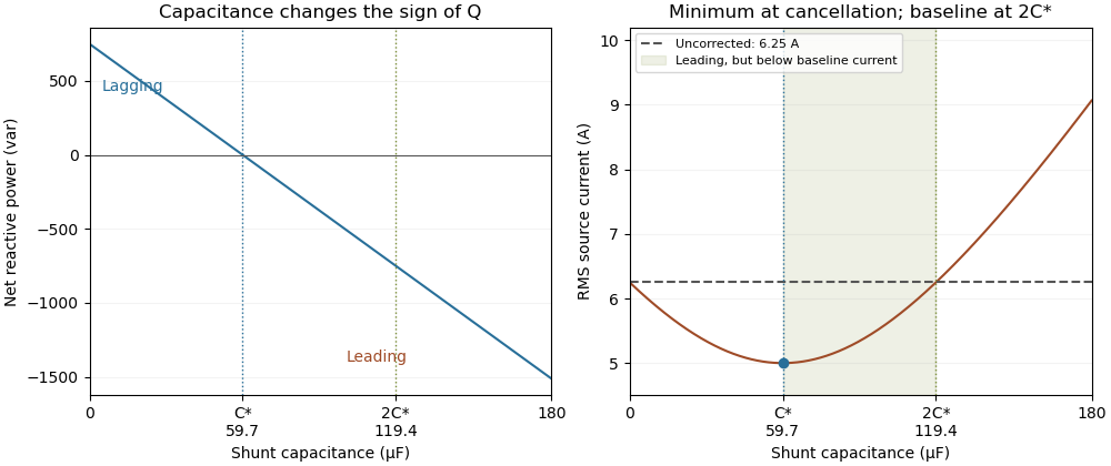
Leading operation begins before correction increases current above the uncorrected value
. Original constant-load model at 200 volts RMS and 50 hertz with 1000 watts active power and 750 vars inductive reactive power. Optimal correction is about 59.68 microfarads. Between 59.68 and 119.37 microfarads the source is leading but still draws less current than the uncorrected load; above 119.37 microfarads it draws more. Details.The optimum changes with the load. If the example load's and both halve while its original optimal correction remains connected, then and . Source electric current is 3.125 amperes and the factor is 0.8 leading. This dependence motivates automatic power factor correction. The cited controller description measures system electric potential difference and electric current, using external current transformers, and switches discrete capacitor bank stages to follow a target.[ref]
Retain the phase or sign of when reporting the result. A bare power factor magnitude does not distinguish leading from lagging; the manufacturer FAQ also illustrates how a meter's signed display depends on its convention.[ref]
Power factor sign conventions in Schneider Electric FAQ FA212521. Resolution and displayed IEC/IEEE convention diagrams
The calculation assumes sinusoidal steady state; current distortion factor is a separate consideration for nonsinusoidal current.Optimal shunt capacitance for sinusoidal power factor correction minimizes the source's RMS electric current for an ideal fixed sinusoidal supply and a fixed load with active power and inductive reactive power . A lossless parallel capacitor supplies signed reactive power , where is the supply RMS electric potential difference and the angular frequency.
The squared source electric current isDifferentiating givesThus the unique minimum isThe fundamental quadrature electric current vanishes there. Strict convexity proves this is a global optimum in the stated model, rather than merely a stationary point. The capacitive sign and one-frequency complex electrical power relation follow from the primary MIT derivation.[ref]
AC Power Flow in Linear Networks by James L. Kirtley Jr.. Energy and Power, equations 61–65 and 71; §7.1 RMS amplitudes
For an original example, , , and give . Source electric current falls from to . A capacitance 20% below or above leaves or , respectively, and both draw about . They have the same power factor magnitude, about , but opposite lead/lag direction.
The exact excess above the optimal squared electric current isSmall sizing errors therefore affect this loss objective quadratically around the optimum, while residual reactive power changes linearly and changes sign. An allowed interval clips the optimum to its nearest feasible point. If the original load has , the constrained optimum for added nonnegative capacitance is instead .
The result assumes a fixed load, ideal sinusoidal supply, lossless correction and no additional network effects. It does not optimize a system with waveform distortion, component heating, variable terminal electric potential difference or discrete stages. The current reduction interval for shunt reactive compensation describes a wider set of beneficial choices, while automatic power factor correction follows a changing load with available stages.
Automatic power factor correction adjusts a correction device as the measured load changes, rather than leaving one fixed compensating setting connected. In a staged capacitor bank, a controller uses terminal electric potential difference and electric current information to choose which stages are connected. The controlled quantity and target must distinguish active power, signed reactive power, waveform distortion and the chosen lead/lag convention.
For an original single-phase sinusoidal model, available stages each supply of capacitive reactive power at the operating electric potential difference. With connected stages,At fixed , maximizing the magnitude of the power factor chooses the available integer minimizing . Away from the end limits, nearest-stage rounding leaves . This capacitor-stage quantization error can be positive or negative. A policy forbidding leading operation instead restricts , so it can choose a different setting.
Suppose , and . Three stages leave and factor about leading; two stages leave and factor about lagging. Both outcomes are consistent with their respective objectives. If the load changes to , , leaving all three stages connected produces ; zero stages is closer to cancellation than one. A stored stage decision must therefore be updated when the load changes.
Actual feedback must measure the corrected network. The Eaton paper places the current transformer so it senses the relevant load and capacitor contribution, and explains how a wrong phase, polarity or location produces misleading feedback.[ref]
Capacitor Application Issues by Thomas M. Blooming and Daniel J. Carnovale. Section VI.C, printed p.8, CT Location for Automatic Banks
Measuring only the correction branch would not establish the combined source power factor.A proposed controller test varies a known resistive-inductive load through several operating points, recording stage state, signed reactive power, RMS electric current and synchronized terminal waveforms. Check both increasing and decreasing demand, including small excursions around a stage threshold. A dead band and timing rules can prevent repeated switching in response to small fluctuations; they must be specified along with the target. Stage size, switching transients and the load's harmonic components require additional checks beyond the ideal rounding model.
Rotation-axis direction uncertainty in clearance bounds accounts for a robot rotating about a direction different from the modeled direction. Even an exactly located pivot does not determine the final occupied geometry if its axis direction is uncertain. Rotation acts through a rotation matrix; Rodrigues rotation formula computes that matrix from a unit axis and rotation angle.[ref]
Modern Robotics: Mechanics, Planning, and Control by Kevin M. Lynch and Frank C. Park. §3.2.3, Exponential Coordinates of Rotation, Part 2, Rodrigues formula
Assume the pivot and principal rotation angle are known and shared by both models. Let the unit axes be , separated by , and suppose every occupied point obeys . The endpoint discrepancy isIt measures error against a nominal endpoint, not total motion from the initial position.
One exact operator norm calculation uses the unit quaternions and its modeled counterpart. Their scalar product isThe relative rotation has half-angle cosine . A rotation through angle moves a perpendicular unit vector by , givingConsequently, if the direction error is at most ,The cap follows because both endpoints lie on the same radius- sphere. The bound vanishes at zero rotation and, for small axis error, scales approximately as . Opposite oriented axes represent the same rotation at ; the conservative inequality need not capture that special cancellation.
For an original rotary-tool example, , and give an endpoint-error allowance of , about . A direction tolerance that looks small numerically can consume a substantial clearance margin at a long tool tip.
A combined pivot and axis uncertainty in rotational clearance must add or jointly bound pivot-location error, angle error and direction error without double-counting a shared coordinate-frame error. The fixed-axis formula in pivot-location uncertainty in a rotational clearance bound addresses a different contribution. For a proposed test, observe multiple rigid fiducials over several angles, fit pivot and direction, and validate independent endpoint measurements against the claimed enclosure. Geometric robot motion planning needs the resulting occupied-body bound along the path, rather than only at its final orientation.[ref]
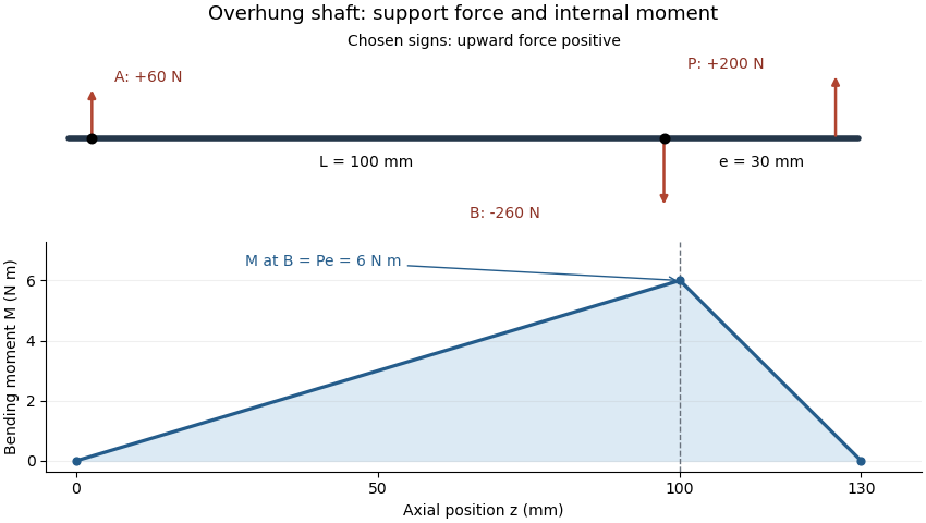
An overhung shaft bending moment is the internal bending moment produced when a transverse load acts beyond the shaft's support span. For a single end load at overhang distance , its magnitude immediately next to the nearer support isin the ideal two-support shaft model. The relevant lever arm is the distance beyond that support, rather than the distance between supports. Manufacturer bearing-load guidance distinguishes this arrangement from a load located between bearings.[ref]
Place ideal supports A and B at axial positions and , and apply an upward load at . With upward reactions positive, static equilibrium givesChoosing the internal moment sign consistently with the left-hand force sums, the bending moment along the shaft isIt is continuous at B, reaches there and vanishes at the free end. An ideal bearing need not apply a concentrated couple for the shaft's internal moment at its location to be nonzero: the shaft continues beyond that support.
For original values , and , the reactions are and and the peak moment is . Doubling at fixed doubles that moment. Changing while keeping fixed changes the reactions but leaves unchanged.
For a uniform solid circular shaft in simple elastic bending, overhung shaft bending stress follows from and :At diameter , the example gives about . This excludes stress concentrations and other loads; a shaft's allowable load requires more than this nominal estimate. Bending can remain even when opposing gear torques give zero net shaft-axis torque, because transverse-force moments and axial twisting are different components of the mechanical loading.
Near-null directions of a pressure sensor array are changes of a modeled pressure field that produce small, rather than exactly zero, changes in the sensor outputs. They distinguish an ill-conditioned reconstruction from the exact ambiguity in the null space of a spatial pressure measurement. A formally invertible response can still contain very little usable information about some pressure patterns.
Choose a finite basis for the pressure field and a linear response , where contains pressure coefficients, the readings, and measurement error. With common pressure units for the coefficients and readings, letbe a singular value decomposition. A change changes the noiseless readings by . Inverting that component divides the measurement error by . If the errors have covariance , the standard deviation of the reconstructed coefficient along is . An exact zero gives no inverse; a small nonzero value gives noise amplification.
An original two-region example has uniform pressures and sensor matrixBoth sensors mostly measure the same average. Write and . Then and . Uniform pressures give readings ; the markedly different pair gives only . The matrix is invertible, but these outputs differ by just in one channel.
If each channel has independent standard uncertainty, the direct contrast estimate is , with standard deviation about . The matrix’s smallest singular value is approximately , consistent with roughly uncertainty in the unit-length contrast direction. Nonnegative pressure constraints can restrict the admissible answers, but do not turn these noisy readings into precise contrast information.
Numerical rank depends on a chosen tolerance. SciPy’s pinned null-space implementation compares singular values with a relative cutoff and returns right singular vectors beyond the retained rank.[ref]
SciPy 1.16.2 documentation. v1.16.2 scipy/linalg/_decomp_svd.py, null_space, docstring and lines 395–403
A floating-point cutoff detects numerical scale; a physical decision about usable information must also consider sensor noise, response uncertainty and the chosen pressure basis. Rescaling a coefficient can change a raw singular value without changing the apparatus.A noise-whitened pressure sensing matrix accounts for unequal or correlated measurement errors before comparing response strength. For positive-definite error covariance , analyze together with the same coefficient units and normalization. A duplicate noisy channel does not provide the same information as an independent measurement of the weak contrast.
Tikhonov regularization can limit amplification by using factors instead of . Relative to the true noiseless coefficient, this introduces attenuation . For and , that factor is about : the weak component is nearly suppressed. A smoother map can therefore have less noise while omitting real contrast. A proposed validation applies independently known pressure patterns that excite both average and contrast directions, repeats the measurements, and reports the error covariance and response-model uncertainty alongside reconstruction results.
A neural network channel indexes a component or response type at each position of a neural network's data grid. In a two-dimensional convolutional neural network, the channel axis is distinct from the two spatial axes. For example, an image represented with the RGB color model has red, green and blue input channels, while an intermediate neural network feature map can have many learned response channels.[ref]
Conv2d in the PyTorch documentation. Opening equation, input/output channel counts and spatial dimensions
The arrangement of axes must be stated. In the documented convention , counts examples, channels, rows and columns. Thus two three-channel images, each four pixels high and five pixels wide, have shape and containscalar entries. Changing the number of examples does not change the number of channels in each example.[ref]
Conv2d in the PyTorch documentation. Shape, batched input convention
A dense convolutional layer can mix all input channels into each output channel. For the preceding input, use eight output channels, three-by-three filters, convolution stride one and no padding. The output shape iswith scalar entries. Its eight filters use weights, plus eight biases if enabled, giving parameters. The leading example count does not multiply this parameter count: the same weights process each example.[ref]
Conv2d in the PyTorch documentation. Opening channel-summation equation; Shape; Variables, dense weight and bias dimensions with groups=1
The eight output channels are not eight new primary colors. Their values are determined by learned combinations of the preceding channels and spatial neighborhoods. Individual channels can be useful for interpretation, but a channel's index does not by itself identify a human-named feature or make its response a probability.
A pointwise convolution makes the channel operation especially clear: at every spatial point it maps one channel vector to another using the same matrix of weights. By changing that matrix, it can reduce or increase the channel count while preserving the grid dimensions under unit-stride, unpadded conditions. Keeping channel, spatial and example axes separate prevents both shape errors and misleading interpretations.
Pinned article: Introduction to the OurBigBook Project
Welcome to the OurBigBook Project! Our goal is to create the perfect publishing platform for STEM subjects, and get university-level students to write the best free STEM tutorials ever.
Everyone is welcome to create an account and play with the site: ourbigbook.com/go/register. We belive that students themselves can write amazing tutorials, but teachers are welcome too. You can write about anything you want, it doesn't have to be STEM or even educational. Silly test content is very welcome and you won't be penalized in any way. Just keep it legal!
Intro to OurBigBook
. Source. We have two killer features:
- topics: topics group articles by different users with the same title, e.g. here is the topic for the "Fundamental Theorem of Calculus" ourbigbook.com/go/topic/fundamental-theorem-of-calculusArticles of different users are sorted by upvote within each article page. This feature is a bit like:
- a Wikipedia where each user can have their own version of each article
- a Q&A website like Stack Overflow, where multiple people can give their views on a given topic, and the best ones are sorted by upvote. Except you don't need to wait for someone to ask first, and any topic goes, no matter how narrow or broad
This feature makes it possible for readers to find better explanations of any topic created by other writers. And it allows writers to create an explanation in a place that readers might actually find it.
Figure 1. Screenshot of the "Derivative" topic page. View it live at: ourbigbook.com/go/topic/derivativeVideo 2. OurBigBook Web topics demo. Source. - local editing: you can store all your personal knowledge base content locally in a plaintext markup format that can be edited locally and published either:This way you can be sure that even if OurBigBook.com were to go down one day (which we have no plans to do as it is quite cheap to host!), your content will still be perfectly readable as a static site.
- to OurBigBook.com to get awesome multi-user features like topics and likes
- as HTML files to a static website, which you can host yourself for free on many external providers like GitHub Pages, and remain in full control

Figure 2. You can publish local OurBigBook lightweight markup files to either OurBigBook.com or as a static website.
Figure 3. Visual Studio Code extension installation.
Figure 5. . You can also edit articles on the Web editor without installing anything locally. Video 3. Edit locally and publish demo. Source. This shows editing OurBigBook Markup and publishing it using the Visual Studio Code extension. 
- Infinitely deep tables of contents:




All our software is open source and hosted at: github.com/ourbigbook/ourbigbook
Further documentation can be found at: docs.ourbigbook.com
Feel free to reach our to us for any help or suggestions: docs.ourbigbook.com/#contact