Topics (384k) Articles (398k) Users (410) Discussions (242) Comments (383) Files (13k) New article

Thermal-product dependence beyond covariance is the influence of higher joint moments on uncertainty in a nonlinear thermal expansion correction. Two input models can have identical means, variances and covariance yet predict different uncertainty in a product. A thermal-product input-distribution check must therefore examine how the temperature offset and expansion-coefficient error occur together.
Let and , where the centered variables have expected values zero, variances and covariance . Direct expansion givesThe third joint moments and the mixed fourth moment of thermal inputs are extra information. For centered inputs, only the last two terms remain. A first-order uncertainty propagation rule at zero input means would miss the product entirely; the GUM explicitly requires higher-order treatment when nonlinearity matters.[ref]
An original counterexample keeps even the marginal shapes fixed. Let have a standard normal distribution and let independently take values and with equal probabilities. Define and . Both have centered normal distributions, the quoted variances and zero covariance. They are not independent: their absolute standardized values are identical.
Their product is . Its expected value is zero, while its variance is , because . Independent centered normal inputs with the same individual variances instead give product variance . The joint model, rather than a marginal histogram or correlation coefficient alone, determines the difference.
For an illustrative length correction with zero means, , and , these models give standard deviations nm and 10 nm. This constructed dependence is a mathematical test case, not a proposed universal thermometer model.
In a physical gauge block study, track paired temperature and coefficient information, shared thermometer corrections and any procedure that estimates one input using the other. NIST's thermal correction explicitly combines block length, expansion coefficient and temperature difference.[ref] Preserve that dependence when generating joint draws. JCGM 101 distinguishes model formulation from propagation and gives a multivariate Gaussian input model as a specific choice, not a consequence of normal marginals alone.[ref] More simulation trials reduce numerical error conditional on the chosen model; they cannot identify unmeasured joint moments.
A Suzuki ovoid is a special set of points in the three-dimensional projective space over , for . It is an ovoid: no three of its points are collinear. Its projective symmetries include the Suzuki group of Lie type , acting two-transitively on these points.
For , fixing one point leaves a stabilizer of order , with a subgroup of order acting regularly on the other points. Thus the geometry realizes the natural permutation action of the group, rather than only its four-dimensional matrix action. For , there are ovoid points and .
The absence of collinear triples means that choosing two ovoid points determines a secant containing exactly those two ovoid points. There are therefore such secants. This turns part of the geometry into an explicit pair-counting problem.[ref]
On the simple groups of Suzuki and Ree by Robert A. Wilson. Introduction and section4.1, Suzuki ovoid and natural doubly transitive action
The sheaf of total quotient rings, or sheaf of meromorphic functions, of a scheme is constructed by locally allowing denominators that are nonzerodivisors. For an open set , let consist of sections of whose germ is a nonzerodivisor at every point of . Sheafifying the presheafgives . The stalkwise regular-denominator condition ensures that restriction to smaller open sets is defined. Merely taking arbitrary fraction rings of section rings is not a substitute for this construction.[ref]
The Stacks project. Tag01X1, Definition31.24.1
For a locally Noetherian scheme, is the total quotient ring of , and on an affine open its sections are the total quotient ring of . These identifications require the stated hypothesis.[ref]
The Stacks project. Tag0EMG, Lemma31.25.2
For an integral scheme this recovers its field of rational functions locally. For , every nonzerodivisor is already a unit, so its total quotient ring is itself and retains a nonzero nilpotent. Total quotient rings therefore need not be fields or remove infinitesimal structure.
A microplate reader is an optical instrument that records signals from addressed wells in a microplate, allowing many small samples, references and repeats to be measured in one arrangement. In absorbance mode it acts as a spectrophotometer: wavelength-selected illumination passes through the well and a photodetector measures transmitted light. The vertical sample geometry makes the liquid depth part of the optical path length.[ref]
For an ideal homogeneous non-scattering solution, the Beer-Lambert law giveswhere is the geometric light path through the solution. For an original dye example, suppose . A0.50cm depth gives absorbance0.30 and transmittance about0.501, whereas a1.00cm depth gives absorbance0.60 and transmittance about0.251. The concentration is identical. A darker well can therefore result from a longer path rather than a more concentrated sample. Microplate path-length correction is needed when comparing such readings on a common path-length basis.
A manufacturer experiment used a yellow buffer at426nm in a96-well clear plate, with volumes from75 to300µL. A1cm cuvette gave absorbance0.556. Uncorrected plate values were roughly0.17–0.53, while path-length-corrected values ranged from0.55 to0.57. The varied-volume experiment directly illustrates why the raw signal cannot be interpreted as concentration alone.[ref]
Optical density measurements automatically corrected to a 1-cm pathlength with PathCheck Technology by Molecular Devices. “Experimental Results”, Figures7,9–10
The same instrument technology estimates path length using water's near-infrared absorbance at1000 and900nm, with plate-background subtraction preceding normalization.[ref]
Optical density measurements automatically corrected to a 1-cm pathlength with PathCheck Technology by Molecular Devices. “Principles of PathCheck”; “Failure to perform appropriate background subtraction”
In a simple independent example, a sample reading0.34 with plate contribution0.04 leaves solution absorbance0.30. At path0.50cm, normalization to1cm gives0.60. Dividing the uncorrected0.34 by0.50 instead gives0.68, incorrectly assigning the plate's contribution to the solution.The instrument must therefore preserve well positions, wavelength settings, reference measurements and the reduction applied to each reading. Blank correction, matched sample handling and appropriate measurement calibration help distinguish optical differences from differences in concentration. A microplate reader can produce an array of precise numbers while a shared path-length or background error affects the whole array.
Raman spectral rebinning with conserved integrated counts redistributes finite-bin measurements onto a new spectral grid while preserving their summed quantity over the same covered range. It is different from relabeling bin centres or interpolating peak heights. The parent spectral-density conversion between wavelength and Raman shift derives the continuous Jacobian; finite bins require a stated assumption about unresolved variation inside each bin.
For an original piecewise-constant wavelength-density model, let old bin have width and count . Invert the new Raman-shift edges to wavelength intervals . Define the overlap matrixWhen the new bins partition the old covered range, , hence . Clipping the new range instead excludes the corresponding counts and must be reported.
For original old wavelength bins and with counts and , choose new edges corresponding to wavelengths , , and . ThenThe total remains . A different within-bin model can distribute that total differently; the original measurements do not resolve every sub-bin feature.
Covariance of count-conserving rebinned Raman channels transforms as for this fixed linear operation. Fractional rebinned estimates are therefore not automatically independent Poisson photon counts. Splitting one measured bin among neighbours creates shared uncertainty; finer output pixels do not create additional spectral resolution.
The primary FSRS instrument records a dispersed spectrum on an array and calibrates its Raman-shift axis.[ref]
Femtosecond Broadband Stimulated Raman: A New Approach for High-Performance Vibrational Spectroscopy by David W. McCamant and others. Instrumentation/Figure 2 and absolute-shift calibration; Data Collection
The overlap algorithm above is an original illustrative reconstruction, not a claim about that instrument's published processing. Apply radiometric response and background corrections consistently with the quantity whose integral is being conserved.Unequal spectral offset sensitivity occurs when a shared instrumental or reference offset influences two spectral estimates by different amounts. It limits spectral common-mode offset rejection: subtraction cancels a common disturbance only to the extent that its two response coefficients match.
For frequencies , write an explicit measurement modelwhere is the shared offset, are dimensionless sensitivities and are residual errors. ThenThus even perfectly shared leaves a residual when .
An original uncertainty example uses , and standard uncertainty . The offset contribution to the difference is . With independent residual standard uncertainties of each and no correlation with , the combined uncertainty isA general calculation retains the relevant covariances; the independent-error simplification is an assumption, not a consequence of a shared instrument.[ref]
Evaluation of measurement data — Guide to the expression of uncertainty in measurement by JCGM. Section 5.2, correlated-input propagation and sensitivity coefficients
Reweighting also changes what is measured. Subtracting from cancels when both sensitivities are nonzero, but estimates , not generally the original frequency difference. Achieving cancellation is insufficient unless the resulting estimator still answers the intended physical question.
A controlled reference perturbation can estimate the slopes and while the true spectral features are held stable. Their difference predicts leakage. Spectral offset identifiability asks whether the available observations can distinguish a real change of frequency separation from this leakage; one observed difference alone cannot determine both an unknown physical change and an unknown offset. Reference features, controlled perturbations or independently established response coefficients supply additional information.
The null space of a spatial pressure measurement consists of changes to a contact pressure field that leave every measured channel unchanged. For a linear response model on a contact region , writeThen . Two fields have identical outputs precisely when their difference lies in this kernel of a linear map. The sensitivity kernels , their support and the admissible class of pressure fields are part of the model.
For an ideal area-average sensor, inside cell and zero elsewhere. A positive and negative perturbation within one cell can cancel in its integral while remaining invisible to the other cells. This is the mechanism behind spatial pressure-map resolution below a sensor cell. It is a nonuniqueness of the observations, even if their numerical values are exact.
An original finite model divides each of two equal-area sensor cells into two equal halves with constant pressures . The observed averages areThis matrix has rank two and a two-dimensional null space spanned by and . Thus the fieldsboth produce . Their peak pressures differ by . Adding an independent measurement of determines the first pair, but still leaves the second pair’s difference undetermined. An extra channel helps only if it adds an independent constraint on the missing directions.
The linear null space is not itself a set of physical pressure fields: its perturbations can have either sign. For a nonadhesive contact, require as well. With the uniform field above, perturbations are admissible for . Positivity restricts the ambiguity without removing it. In contrast, a zero area-average reading together with a nonnegative pressure assumption forces pressure to vanish almost everywhere in that cell under the ideal model.
For a chosen finite basis of pressure fields, a singular value decomposition identifies the matrix null space. SciPy’s pinned implementation constructs its basis from right singular vectors and uses a relative singular-value cutoff to determine effective numerical rank.[ref]
SciPy 1.16.2 documentation. scipy.linalg.null_space, pinned v1.16.2 scipy/linalg/_decomp_svd.py, docstring and implementation lines 333–403
A numerical cutoff and an exact zero singular value are different notions. Near-null directions of a pressure sensor array have small nonzero responses and can amplify measurement error: a dimensionless singular value of turns a channel-error component into a coefficient error when inverted without regularization.A proposed apparatus check applies controlled local loads to estimate the sensitivity kernels, then compares fields with similar predicted channel outputs using independent spatial measurements. Contact area, load spreading and cross-coupling must enter that comparison. A reconstruction algorithm may select one smooth or nonnegative solution, but the selected structure is additional modeling information; it is not automatically an independently observed subcell pressure map.
The uncertainty of a three-point baseline integral depends on both the sample uncertainties and their correlations. With a known fixed gate duration , Simpson baseline integration for pulse-energy correction uses the linear combinationIf is the covariance matrix of the baseline estimates, thenFor fixed weights this variance identity is exact; it does not require Gaussian errors. Its use as a complete measurement uncertainty still requires an adequate baseline model. The general covariance propagation rule retains these cross terms.[ref]
An original equal-precision model assigns each sample standard uncertainty and common pairwise correlation coefficient , with . Substitution givesFor and , independent samples give . At this rises to ; a perfectly common additive error gives . Three readings under one uncertain offset need not behave like independent measurements.
The final corrected pulse integral has another covariance. If is the raw gate integral and , thenThe covariance between a raw pulse integral and its baseline correction matters when both share a readout offset. If that offset is , it contributes to both and and cancels exactly in their difference. Treating these appearances as independent would invent uncertainty.
Use repeated matched blank acquisitions to estimate the relevant covariance structure, keeping the gate and readout sequence comparable. A contaminated midpoint, an inadequate baseline shape or uncertain timing adds effects outside the fixed-weight sample-noise calculation. Numerical quadrature exactness alone does not establish a sound pulse-energy uncertainty budget.
On an oriented Riemannian smooth four-manifold with a Spin-c structure, let be the spinor bundles and their determinant line. The Seiberg–Witten equations couple a unitary connection on and a positive spinor :Here is the Dirac operator, is the self-dual part of the curvature, and is the quadratic spinor map into imaginary self-dual two-forms. Numerical factors and signs in depend on the Clifford conventions; a perturbation adds a prescribed imaginary self-dual two-form.
The first equation is first-order and elliptic, while the curvature equation makes the coupled system nonlinear. Gauge transformations identify equivalent connection-spinor pairs. Solutions with are reducible and satisfy in the unperturbed system.
On closed four-manifolds, suitably perturbed moduli spaces yield the Seiberg–Witten invariant of a four-manifold. The abelian gauge equations arose from the monopole description of supersymmetric gauge theory and provide tools for distinguishing smooth four-dimensional geometry.[ref]
Noise remaining after scaled Raman subtraction is the random uncertainty left when a surface contribution's mean has been cancelled. For two measured spectral channels and fixed scale , scaled subtraction of two spatially offset Raman spectra uses . Its exact variance isThe covariance term describes the actual acquisition relationship; numerical subtraction does not itself make the inputs correlated or independent. General measurement propagation retains such terms.[ref]
A focused extension allows an uncertain subtraction scale , independent of the pair , with mean and variance . Expanding the product's moments givesThe final term includes uncertainty in the reference scale, not just shot noise in the two spectra.
For an original surface-only example, let independent Poisson photoelectron counts have means and , with . The mean residual is zero. A perfectly known scale gives variance and standard deviation . If instead , the variance becomes , giving standard deviation in the scaled count units.
If is estimated from these same counts, the independence assumption needs replacement by the appropriate joint model. A scale shared across wavelengths can also produce correlated spectral residuals from a shared subtraction scale, leaving a structured band-like error rather than independent noise in each bin. The original SORS study demonstrates changing layer contributions with collection offset; the moment calculation here is an independent noise model for a simplified subtraction.[ref]
Subsurface Probing in Diffusely Scattering Media Using Spatially Offset Raman Spectroscopy by P. Matousek and others. Abstract, offset-dependent mixtures and numerical layer separation
Confidence bounds from a samplewise variance bound use a variance comparison that holds for the realized statistic, together with a valid tail inequality. The unbiased two-sided construction is proved in samplewise variance upper bound. A useful extension includes a separately justified bias budget: assumewhere is a validated deterministic bound and the estimator has finite variance. For , defineIf lies outside this interval, the triangle inequality implies . The samplewise bound and Chebyshev's inequality then give . No independence between the centre and is required. Zero true variance is covered because the centre then equals its expectation almost surely.
For an original measurement example in a fixed unit, suppose the reported estimate is , a validated residual-bias bound is , and a deterministic samplewise variance upper bound is . With , the radius isso the interval is approximately . The conclusion applies over repeated measurements under those assumptions. The particular realized interval is not assigned a frequentist probability that the fixed parameter is inside it. Replacing the radius by would discard both the bias allowance and the tail justification.
The bound is an assumption about the centre's possible systematic displacement; a guessed correction uncertainty is not automatically such a bound. NIST distinguishes the coverage interpretation from merely applying a conventional multiplier to a standard uncertainty.[ref]
Guidelines for Evaluating and Expressing the Uncertainty of NIST Measurement Results by Barry N. Taylor and Chris E. Kuyatt. §§6.2–6.3
If only an upper or lower endpoint is required, a one-sided Cantelli confidence bound with a bias budget uses a one-sided inequality rather than silently reusing a two-sided normal critical value.In an ideal unbounded fluid governed by the Boussinesq approximation, take uniform background temperature and salinity gradients , with upward. Let be the thermal expansion coefficient and haline contraction coefficient, and let the thermal diffusivity exceed the solutal diffusivity . With the conventiona strictly stable total mass density gradient has . The band admitting exponentially growing salt fingering modes isThe upper equality is the marginal long-wavelength limit. This local linear stability result assumes no rotation and constant positive kinematic viscosity; finite boundaries can restrict the available wavelengths.[ref]
Double-diffusive processes in stellar astrophysics by Pascale Garaud. Section 2.2.1, equations15–16 and the definition of the density ratio
A dimensional derivation makes the signs explicit. Put and , where is the gravitational acceleration. Consider a normal mode with growth rate , squared wavenumber and horizontal fraction , where is the wave vector and its horizontal magnitude. Eliminating the temperature, salinity and pressure perturbations from the linearized equations gives the characteristic polynomialwhere is the kinematic viscosity.
For an elevator mode, and the perturbation is independent of . Its constant term isIf , choose a sufficiently small positive to make . Since tends to positive infinity along the positive real axis, the intermediate value theorem supplies a positive real growth rate.
For the converse, write . When , all three coefficients are positive, andThe Routh-Hurwitz criterion therefore puts every root in the left half-plane. This covers oblique modes too, since . If , ordinary density-driven overturning is already available; that is a different regime from fingering within a stably stratified background.
An elevator mode is a normal mode whose fluid motion is purely vertical while its velocity, temperature and composition perturbations are independent of height. Neighbouring columns can move upward and downward without a vertical return-flow structure, hence the name. Such modes describe the fastest-growing disturbances in the ideal local salt fingering problem.[ref]
Double-diffusive processes in stellar astrophysics by Pascale Garaud. Section 2.2.1, paragraph following equation 16: vertically invariant elevator modes
Take upward and write the velocity field and scalar perturbations asThe incompressibility condition is automatic because . More surprisingly, the perturbation's own advection of every one of these fields vanishes:The background need not be uniform: if its temperature and salinity gradients are constants , vertical motion still advects those backgrounds. This supplies the terms and below.
In a nonrotating local model with the Boussinesq approximation, constant kinematic viscosity and constant thermal diffusivity and solutal diffusivity , the ansatz reduces the equations toHere is gravitational acceleration, the thermal expansion coefficient, the haline contraction coefficient, and the horizontal Laplace operator. A constant pressure perturbation is compatible with the absent horizontal motion.
For example, let all three fields be proportional to , with . The upward and downward columns alternate with wavelength . Their amplitudes satisfy a three-variable linear differential equation; eliminating the scalar amplitudes gives the characteristic polynomial used in the salt-finger instability criterion. Although that criterion is a linear stability result, the vanishing self-advection means that this particular ansatz also solves the corresponding nonlinear local equations exactly within the stated ideal model.
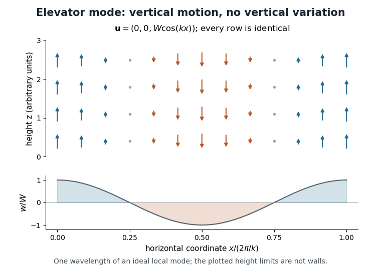
An elevator mode across one horizontal wavelength
. Original schematic with vertical velocity field . Each height has the same pattern of upward and downward motion; the lower plot shows its horizontal profile. The top and bottom of the drawn region are not impermeable walls. Details.That exactness does not imply that unlimited growth describes a laboratory tank. An impermeable horizontal wall requires the vertical velocity to vanish there, excluding a nonzero height-independent pattern. Other perturbations can also grow on the rising and falling columns and disrupt them. Elevator modes are therefore useful ideal building blocks, with boundary conditions and additional disturbances determining how faithfully a real flow follows them.
An RNA relaxation instrument-response correction accounts for the way an experiment's heating, detection and recording alter an underlying molecular transient. A measured RNA melting relaxation time can otherwise combine molecular kinetics with instrumental behavior. The response must be characterized for the actual apparatus and measurement conditions.
For an illustrative linear, time-invariant detector, let the normalized instrument response function be for . Suppose the ideal molecular signal is after excitation, and both vanish before it. Their convolution gives, for ,The recorded trace rises before decaying even though the assumed molecular transient begins at its maximum. Fitting the entire trace as one unblurred exponential would misdescribe the model.
An original example sets and . The measured signal peaks at with height . Its normalized temporal centroid is , rather than 10. These different time summaries cannot be substituted for one another.
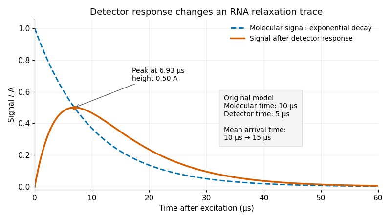
Original exponential RNA transient and its convolution with a finite instrument response function; stipulated molecular time10μs and detector time5μs
. Details. One useful approach predicts a molecular transient, convolves it with the characterized instrument response function, and fits that forward prediction to the data. Directly undoing a smoothing response can amplify measurement noise. Parameters that produce nearly indistinguishable recorded curves may remain difficult to determine separately.
Sample cooling is an additional physical process. A primary temperature jump study used a thin sample cell to accelerate cooling enough to observe RNA refolding, with separate infrared probe pulses following the transient.[ref]
Measuring RNA UNCG Tetraloop Refolding Dynamics Using Temperature-Jump/Drop Infrared Spectroscopy by C. P. Howe and others. Printed pp.9171–9172, thin-cell cooling and pump/probe measurement.
If temperature changes during a trace, the molecular equilibrium and rate constants may change too; detector convolution alone does not account for that changing input. The two-exponential example is a stipulated teaching model, not a fit to that paper.RNA melting log-odds uncertainty quantifies uncertainty in , the transformed population used in an RNA melting log-odds plot. It depends on the unfolded fraction as well as its uncertainty. The transformation becomes particularly sensitive near 0 and 1.
For a sufficiently concentrated uncertainty distribution within , first-order uncertainty propagation givesWith an original stipulated , the standard uncertainty is 0.040 at but approximately 0.510 at . Equal population uncertainties do not justify equal statistical treatment of transformed observations.[ref]
Evaluation of measurement data — Guide to the expression of uncertainty in measurement by JCGM. §5, sensitivity-coefficient method; derivative here follows from the stated logarithmic transformation.
Nonlinearity also creates asymmetry. At , . Changing the fraction to 0.01 gives , while changing it to 0.03 gives : equal changes in fraction produce unequal transformed changes. These are deterministic perturbations, not asserted confidence limits. If the uncertainty materially reaches 0 or 1, the linear approximation needs reconsideration; taking the logarithm of those endpoints is undefined.
The underlying RNA melting baselines can induce shared errors across temperatures. For an optical mixture with ,soThese derivatives propagate the joint uncertainty of the measured absorbance and fitted baselines. Reusing baseline parameters for many observations creates RNA log-odds covariance; merely assigning separate error bars does not remove it.
A fit can model the original absorbance observations and their RNA melting baselines, or handle the transformed data with an appropriate joint error model. Optical curves are fitted quantities in primary melting analyses, rather than direct counts of unfolded molecules.[ref]
Thermodynamic characterization of naturally occurring RNA tetraloops by Justin P. Sheehy and others. Materials and Methods, optical curves and thermodynamic fitting.
Precision in a fitted straight line cannot establish the correctness of the two-state RNA melting model used to interpret it.RNA baseline prediction covariance quantifies how errors in fitted RNA melting baselines link their predicted values at different temperatures. Reusing the same fit parameters creates shared uncertainty; predictions are not independent merely because they are evaluated at different temperatures.
For a linear RNA baseline extrapolation , put . ThenThis relation follows from the covariance of two linear combinations. The diagonal gives a prediction variance; the off-diagonal entries determine how predictions move together.[ref]
An original example assumes independent parameters with and . At temperatures below and above , both prediction variances are , while their covariance is . The correlation coefficient is therefore . A slope error moves the predictions in opposite directions around the reference point, outweighing the common intercept error.
The difference between those two predictions cancels the intercept exactly:Its standard uncertainty is 0.008. Ignoring covariance would give , which is too small for this model. Shared fitted inputs can produce negative as well as positive prediction correlations.
In vector form, a prediction covariance matrix is , with rows of equal to and parameter covariance . A two-parameter fit supplies at most two independent shared-error directions, even if evaluated at a hundred temperatures. Additional independent readout errors contribute their own covariance.
When these predictions are used to infer populations in RNA optical melting, propagate their joint uncertainty rather than only separate error bars. This accounting does not test whether a linear baseline is chemically adequate; curvature or an incorrect pure-state model needs separate evidence.
A shunt resistor is a resistor used to establish a known relation between current and a measured electric potential difference. For current sensing, it is placed in the measured current path, and Ohm's law givesThe voltage-sensing circuit should draw negligible extra current for this simple relation to describe the desired branch current. Its small series voltage drop is often called the burden voltage.
An original example uses and . The sensed drop is50millivolts and Joule heating dissipatesReducing resistance lowers both the burden and dissipation, but also reduces signal relative to a fixed amplifier offset or readout noise. The nominal resistor value alone therefore does not determine measurement quality.
Lead and contact resistance can dominate a low-value shunt. If a10milliohm shunt is inadvertently measured together with2milliohms of current-carrying interconnect, interpreting the total voltage using only the nominal shunt value overestimates current by20percent. Four-terminal sensing separates the high-current connections from the voltage-sense connections. Analog Devices' LTC6115 data sheet illustrates these Kelvin sense paths and explains how interconnect resistance introduces error.[ref]
A practical characterization drives known currents through the shunt while measuring the voltage at its sense terminals, then repeats after thermal settling. Temperature coefficient of resistance, self-heating and connection geometry affect the realized conversion. The amplifier's operating range and measurement calibration must be assessed alongside the resistor.
A shunt converts current into a local voltage signal; it does not inherently provide electrical isolation between the measured circuit and its readout. High-side current sensing and low-side current sensing describe alternative placements of that measurement relative to the load and reference conductor.
A reference resistor is a resistor whose assigned electrical resistance supplies the comparison value in a resistance-measurement circuit. Its value may come from measurement calibration rather than its nominal marking. The useful reference is its value under the stated temperature, loading and connection conditions, together with the associated measurement uncertainty.
In a shared-excitation resistance ratio measurement, the sensor and reference resistor carry the same electric current. Measuring their electric potential differences gives , so . A reference value error therefore sets a scale error even when excitation cancels perfectly. Reference-resistor error in ratiometric resistance measurement derives the exact relation and distinguishes a correction from its remaining measurement uncertainty.[ref]
The connections define which resistance is compared. In four-terminal sensing, two leads carry the electric current while a separate high-impedance pair senses the electric potential difference at the reference terminals. This avoids including the current-lead drops in the assigned reference value, within the sensing instrument's limitations.
For an original ideal example, a reference resistor carries through two current leads, each of electrical resistance . The reference element has a potential difference of , while a reading outside both leads is . If this latter reading is used as the denominator while the calculation assumes , a true sensor is inferred asSensing directly at the reference terminals removes this idealized lead contribution. It does not correct a wrong reference value. The circuit guide explicitly shows a Kelvin connection at the reference terminals for this purpose.[ref]
A small temperature change shifts the value approximately by , with temperature coefficient of resistance . Excitation also dissipates electric power ; a reference with a different temperature or load from its measurement calibration may require a correction or additional measurement uncertainty. A proposed check compares the reference before and after the measurement sequence under the same connection and loading conditions. Repeating the comparison at a lower electric current tests for a heating contribution. Stability of the observed ratio alone cannot certify the reference's assigned value.
Reset pedestal variance is the acquisition-to-acquisition variance of the output offset associated with integrator reset. In a model where the only fluctuating contribution is an opening charge on fixed capacitance ,Subtracting the mean of the reset charge-injection pedestal removes its constant component, not the random spread. The physical datasheet distinguishes charge-transfer offset from output noise; its charge-transfer limit alone is not a statistical variance specification.[ref]
ACF2101 Low Noise, Dual Switched Integrator datasheet. p3, Output Noise and Charge Transfer Errors; p11, Charge Transfer
Finite blank measurements introduce another contribution. Suppose independent pedestals have mean and standard deviation . Use independent zero-input acquisitions to estimate , then subtract that same blank sample mean from each of new signal acquisitions. With a constant signal and no other noise, the corrected mean hasThis variance of a pedestal-corrected sample includes the uncertainty of the shared correction. Its second contribution does not shrink when more signal acquisitions reuse the same blank estimate. Covariance-based uncertainty propagation retains such shared terms.[ref]
Guide to the expression of uncertainty in measurement by JCGM. §4.2.3, variance of an arithmetic mean; §5.2.2, correlated inputs
For original stipulated , and , the corrected mean has standard deviation . An exactly known pedestal mean would give . Repeated zero-input acquisitions at a fixed delay after switching measure the combined pedestal/readout spread; separating its mechanisms requires additional tests. Slow drift or correlations between acquisitions invalidate the independent-sample formula and must enter the measurement model.
Finite-perturbation reference sensitivity measures the change in a comparison when one shared reference value is changed by a finite amount everywhere it occurs. It checks both local sensitivity coefficients and their usefulness over the actual reference-uncertainty range. The reference-sensitivity cancellation check is incomplete if it tests only a derivative at one point.
Let be the final comparison, with all other independent inputs held fixed. A central finite difference and a second difference areFor sufficiently smooth , these approach and , with errors of order when the required derivatives exist. Their units differ: comparison per reference unit and comparison per squared reference unit. The GUM defines sensitivity coefficients as partial derivatives and also discusses determining them by varying an input experimentally.[ref]
An original model writes andIt gives and . Comparing with can expose cubic contamination of the local slope. But if , every central slope is exactly zero although is nonzero. A symmetric slope check alone misses an even-in-perturbation response.
For and , the one-sided change is 1 nm, while and . If the shared reference error instead has a zero-mean normal distribution with standard deviation , the quadratic contribution has mean 1 nm and standard deviation approximately 1.414 nm. These are original model calculations. They show why exact cancellation, zero local slope and negligible finite-range influence are distinct claims.
Use step-size stability of a reference perturbation to select a sensible test range. Extremely small steps can magnify numerical subtraction errors; large steps probe a different region of a nonlinear response. Test several scales near the physical standard uncertainty and inspect one-sided changes as well as central slopes. If the model is stochastic, separate simulation noise from the response to the changed reference.
A computational perturbation changes the assigned shared reference in every dependent calculation while keeping its identity shared. Independently perturbing two uses of the same reference changes the covariance model. A physical experiment must additionally hold other influences stable, because changing a standard or its temperature may change contact or instrument behaviour. NIST separates master-block uncertainty from the comparison process in its uncertainty budget.[ref] Retain those physical distinctions when interpreting a numerical sensitivity test.
Pinned article: Introduction to the OurBigBook Project
Welcome to the OurBigBook Project! Our goal is to create the perfect publishing platform for STEM subjects, and get university-level students to write the best free STEM tutorials ever.
Everyone is welcome to create an account and play with the site: ourbigbook.com/go/register. We belive that students themselves can write amazing tutorials, but teachers are welcome too. You can write about anything you want, it doesn't have to be STEM or even educational. Silly test content is very welcome and you won't be penalized in any way. Just keep it legal!
Intro to OurBigBook
. Source. We have two killer features:
- topics: topics group articles by different users with the same title, e.g. here is the topic for the "Fundamental Theorem of Calculus" ourbigbook.com/go/topic/fundamental-theorem-of-calculusArticles of different users are sorted by upvote within each article page. This feature is a bit like:
- a Wikipedia where each user can have their own version of each article
- a Q&A website like Stack Overflow, where multiple people can give their views on a given topic, and the best ones are sorted by upvote. Except you don't need to wait for someone to ask first, and any topic goes, no matter how narrow or broad
This feature makes it possible for readers to find better explanations of any topic created by other writers. And it allows writers to create an explanation in a place that readers might actually find it.
Figure 1. Screenshot of the "Derivative" topic page. View it live at: ourbigbook.com/go/topic/derivativeVideo 2. OurBigBook Web topics demo. Source. - local editing: you can store all your personal knowledge base content locally in a plaintext markup format that can be edited locally and published either:This way you can be sure that even if OurBigBook.com were to go down one day (which we have no plans to do as it is quite cheap to host!), your content will still be perfectly readable as a static site.
- to OurBigBook.com to get awesome multi-user features like topics and likes
- as HTML files to a static website, which you can host yourself for free on many external providers like GitHub Pages, and remain in full control

Figure 2. You can publish local OurBigBook lightweight markup files to either OurBigBook.com or as a static website.
Figure 3. Visual Studio Code extension installation.
Figure 5. . You can also edit articles on the Web editor without installing anything locally. Video 3. Edit locally and publish demo. Source. This shows editing OurBigBook Markup and publishing it using the Visual Studio Code extension. 
- Infinitely deep tables of contents:




All our software is open source and hosted at: github.com/ourbigbook/ourbigbook
Further documentation can be found at: docs.ourbigbook.com
Feel free to reach our to us for any help or suggestions: docs.ourbigbook.com/#contact