Topics (384k) Articles (398k) Users (410) Discussions (242) Comments (383) Files (13k) New article

Optimizer restart equivalence means that restoring an optimization checkpoint reproduces the uninterrupted optimizer's parameter sequence for a specified subsequent computation. State the optimizer update rule, continuation inputs and intended notion of equality. Exact mathematical equality and agreement within a numerical tolerance are different claims.
For a deterministic algorithm modeled by , equality of the restored full state at step , together with the same update rule and future inputs , is sufficient. One application of gives equal next states; mathematical induction then gives equal continuations. This is a sufficient condition for the chosen observations, not a claim that every internal field must always affect them.
For an original exact example, take andFrom , one step gives . Restoring that pair gives and , exactly as uninterrupted execution. Resetting the buffer while restoring gives and . Thus a parameter-only save is not restart-equivalent for this recurrence.
Practical checkpoints must also retain the optimizer state-to-parameter association and the relevant settings, update position, learning rate schedule, data position and pseudorandom number generator state.[ref]
Saving and Loading Models in the PyTorch tutorials. General checkpoint for resuming training: model and optimizer dictionaries and training position
Fixing a random seed alone does not specify all of this continuation. Floating-point arithmetic and nondeterministic operations can additionally affect exact reproduction across environments; the primary documentation does not guarantee identical results across releases or platforms.[ref]Reproducibility in the PyTorch documentation. PyTorch2.15, opening reproducibility statement and controlling randomness
Optimizer state-to-parameter association identifies which parameter each saved piece of optimizer state belongs to. An optimization checkpoint can contain every stored number and still resume incorrectly if those numbers are attached to different parameters. Equal shapes and data types do not establish mathematical identity.
The PyTorch optimizer dictionary separates per-parameter state from parameter-group settings. Its loader pairs saved parameter identifiers with the current parameters in group order, without independently verifying the intended association.[ref]
torch.optim in the PyTorch documentation. PyTorch2.15, Optimizer.state_dict, state/param_groups and loading note
For an original two-parameter example, use and . Let the named parameters be and , their current gradients both be 1, and their saved momentum buffers be and . Correct restoration givesIf a reversed parameter ordering attaches the same saved buffers to the wrong scalar parameters, the result is insteadBoth buffers had valid scalar shapes, so a shape check would not expose this error.
Consistently permuting the parameters, gradients and state is merely a change of ordering; permuting only the state changes the algorithm's continuation. Record a stable parameter schema and group order with the checkpoint, and check any intentional remapping against that schema. Parameter values and optimizer dictionaries are distinct saved objects, so restoring one does not automatically restore the other's meaning.[ref]
Saving and Loading Models in the PyTorch tutorials. What is a state_dict?; Saving & Loading a General Checkpoint
Residual-offset uncertainty in nail thickness estimates is the uncertainty contributed by an imperfectly known additive background after correction of spectral signals. It differs from a known uncorrected offset's bias: subtraction can remove the best estimate of a background while leaving uncertainty about that estimate.
For an original reduced optical model, let two measured normalized signals be and subtract the same background estimate . Define and suppose the attenuation contrast is known. The inferred nail plate thickness isIts sensitivity coefficients areWith mutually independent raw signal estimates and background estimate, first-order uncertainty propagation givesThis follows the sensitivity-and-covariance approach in the measurement guide.[ref]
Guide to the expression of uncertainty in measurement by JCGM. §§5.1–5.2, propagation of input uncertainties and correlated quantities
For stipulated , , , and , the estimated thickness is approximately 0.5108 mm and its combined standard uncertainty is 0.0177 mm. The common-background contribution alone is 0.0133 mm. Averaging 100 independent repetitions of each raw signal while reusing the same background estimate reduces the total only to about 0.0134 mm; it does not reduce that shared contribution by ten.
An equivalent calculation treats corrected signals as correlated: under the stated independence assumptions. Omitting this covariance would describe a different experiment with independent background errors. Near zero corrected signal, the logarithm also becomes strongly nonlinear, so this local approximation needs further checking.
The primary nail experiment included a fluorescence correction in its optical transmission measurement.[ref]
The transmission of optical radiation through human nails by S. G. Parker and B. L. Diffey. Abstract, fluorescence correction
Background emission and dark current must be characterized separately when they have different spectral responses. The equations above are an illustrative uncertainty budget, not a validated thickness calibration or reported precision from that experiment.Nested contact-study allocation chooses how many independent contacts to prepare and how many readings to take within each contact. In a nested wringing-repeatability study, new contacts sample between-wring variability, whereas extra readings of one unchanged contact mainly reduce readout scatter.
For wrings and readings per wring, suppose independent between-wring variance is and independent readout variance is . The overall mean hasAn original planning model assigns cost to preparing a wring and cost to each reading. With fixed budget , a continuous relaxation givesFor positive costs and nonzero , differentiating with respect to yieldsThis balances the cost of new contacts against the benefit of repeated readings. It is not a universal required replication count; integer counts, minimum study sizes and other constraints still apply.
For stipulated costs 9 minutes per wring and 1 minute per reading, with , and budget 180 minutes, the continuous optimum is nine readings per wring. Ten wrings then fit exactly, giving standard deviation for the mean. Eighteen wrings with one reading each give about 1.491 nm; four wrings with thirty-six readings each give about 1.118 nm.
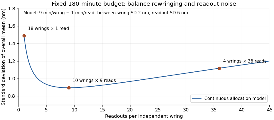
Original fixed-budget model comparing rewringing with repeated readout; all costs and variance components are stipulated
. Details. The variance components need pilot information. Wringing-allocation pilot uncertainty can change the preferred allocation, especially if a small pilot wrongly suggests negligible between-wring variation. Include enough independent preparations to assess that level rather than optimizing solely for an assumed mean variance.
The physical contact can also change with time, handling or surface damage. NIST documents dependence of wringing films on conditions and elapsed time.[ref] Drift, preparation trends and shared reference uncertainty require additional terms; they do not necessarily decrease by adding readings according to this independent-effects formula. State the objective and the constraints with the final design.
Cohomology and base change asks whether changing the base of a family commutes with taking its sheaf cohomology. For a scheme over a ring , an -algebra , and a quasi-coherent sheaf , the natural comparison isHere is the pullback. The left side first computes cohomology and then changes scalars; the right side changes the geometric base first.
Flat base change gives an isomorphism for every when is flat and is quasi-compact and quasi-separated. On separated schemes, the mechanism is a Čech complex from a finite affine cover: flat tensor product preserves the kernels and images needed to compute its cohomology.[ref]
Without flatness, tensor product need not commute with cohomology. The two-term complex in degrees zero and one has zero degree-zero cohomology, but tensoring with makes the differential zero and produces a nonzero degree-zero group. This illustrates the algebraic obstruction; proper-family base-change theorems impose additional hypotheses to control it.
For a morphism of schemes and an -scheme , the Weil restriction is the functor defined on -schemes byWhen this functor is represented by a scheme, that representing object is also called the Weil restriction. Representability needs hypotheses; it is not part of a formal guarantee for every and every base map.[ref]
For , restricting the affine line gives . Indeed, a complex coordinate is expressed as , and for any real algebra the corresponding points are . The construction expresses geometry over an extension field using coordinates over the smaller field, while retaining its full point functor.
An exponentially weighted gradient history assigns geometrically decreasing coefficients to older supplied gradients. For constant and momentum buffer recurrence ,Each additional update multiplies an old contribution by . The formula follows by substituting the expression for into the recurrence and adding the newest exponent-zero term. The same undampened recurrence, including its initialization convention, appears in the primary stochastic gradient descent documentation.[ref]
SGD in the PyTorch documentation. PyTorch2.15, momentum algorithm and first-buffer initialization note
For an original example, choose , and gradients , , . Successive buffers are 2, −1, 3.5. Directly expanding the third buffer givesThe newest contribution has coefficient 1; the oldest has coefficient 1/4. The buffer is a weighted sum, not yet a weighted mean. At , its coefficient sum is the geometric seriesHere , so the normalized weighted mean is , rather than the ordinary mean .
The coefficients also give a concrete memory scale. In the infinite geometric sequence, the fraction assigned to the newest gradients is . At , 29 gradients account for at least 95% of that coefficient mass, because whereas . This is a statement about coefficients, not a guarantee that gradients at different times are independent or that the optimizer averages a stationary process.
A momentum buffer can retain enough earlier history that it points against the current gradient. For the undampened rulethe parameter step is for positive learning rate . If , then the directional derivative in direction is . The actual update direction is therefore locally uphill for a differentiable objective function, even though gradient descent would use the opposite direction. This history-dependent recurrence is the non-Nesterov momentum convention documented for stochastic gradient descent with dampening and weight decay disabled.[ref]
For an original scalar example, let , current , stored buffer , coefficient and . The new gradient is 1, butThe objective increases from to . This is a fully specified finite step, not only a first-order prediction.
More generally,An old buffer sufficiently opposed to the new gradient makes this negative. At , that mechanism disappears. The example explains why a momentum method need not decrease the objective at every step; it does not imply that retaining gradient history always harms convergence. A descent direction test concerns the direction at the current point, while a convergence claim concerns an entire sequence.
A mineralogist studies minerals through their composition, crystal structure, properties and formation conditions. Identifying a specimen requires distinguishing observable appearance from the underlying atomic arrangement: different minerals can look similar, while one mineral can occur in many colors.
X-ray diffraction constrains repeating crystal structure, spectroscopy probes composition and bonding, and controlled heating or pressure experiments test stability ranges. Combining these measurements connects an individual mineral grain with the physical and chemical history of the rock or planetary material in which it formed.
Beam compliance from two support spans separates a cubic span-dependent beam response from a span-independent contribution to the measured mechanical compliance. Assume the same uniform specimen, unchanged machine contribution and a small-deflection central-load model:Here is beam flexural rigidity and . The midspan compliance of a simply supported beam contains the basic numerical fit, while the beam source derives the cubic dependence.[ref]
Beam Displacements by David Roylance. Introduction; Example1, equation7
An original uncertainty example shows why distinct spans can still be too close. Let the actual model have , hence . Assign independent compliance standard uncertainties , and neglect span uncertainty for this example. Since the slope estimate is linear in the readings,Spans and give , about54percent of the actual coefficient. Using and instead gives about3.57percent with the same readout uncertainties. The close-span subtraction strongly amplifies those errors. At the larger relative uncertainty, simply treating as approximately linear is unreliable.
This conditioning of two-span beam compliance inference concerns measurement precision, separately from model adequacy. If shear adds a term proportional to , then has three unknown coefficients that two readings cannot identify. Changing contact or fixture compliance can likewise violate the assumed constant . Further spans and an independent deflection readout test those assumptions; two fitted points alone do not.
Mechanical power-port orientation specifies the signs of the conjugate variables used to describe entering power at a mechanical power port. For a translational port with signed force and velocity , use for net supply into the chosen system. Reversing the coordinate axis reverses both variables, so . Reversing just one variable instead changes the entering-versus-leaving convention and must be stated explicitly. This bookkeeping makes a mechanical supply rate meaningful in a mechanical dissipation inequality.[ref]
Dissipative Dynamical Systems, Part I: General Theory by Jan C. Willems. Storage/supply formulation and power-neutral interconnections
For an element acted on by terminal forces and terminal velocities ,Exchanging terminal labels gives and , preserving power. For , and , both descriptions give . Taking force from the exchanged convention while retaining the original relative velocity would incorrectly report .
More general coordinate changes require the corresponding conjugate-force change. If physical displacement coordinates satisfy , then . Equality of virtual work, or instantaneous power, requiresFor the scalar coordinate , the generalized force is . Thus and correspond to and , both giving1W. Merely rescaling the motion channel without its conjugate force changes the apparent power. At an ideal connection, equal terminal velocities and opposite entering forces cancel internal port powers, enabling the combined mechanical energy balance.
Mechanical dynamic condensation eliminates selected coordinates from a frequency-dependent mechanical response while retaining their effect on the remaining coordinates. It is exact algebraic elimination at the chosen transform variable when the eliminated block is invertible. It is not equivalent to clamping those coordinates. Starting from the partitioned mechanical dynamic-stiffness matrix,solve the internal equation as . Substitution givesThe effective matrix is a Schur complement; the right side is the condensed mechanical load vector. Both matter when the internal coordinate is externally forced. The coupled dynamic equations and measurement boundary conditions are the starting model, rather than independent scalar stiffness reciprocals.[ref]
Structural Testing Part I: Mechanical Mobility Measurements by Ole Døssing. Printed p.11, coupled analytical mechanical models; pp.14–16, force/response descriptions
For the two-mass example at , take and . With and , eliminating coordinate2 gives effective stiffness and effective load . Hence . Omitting the load correction would incorrectly predict no response at coordinate1.
For constant original mass matrix, damping and mechanical stiffness matrix, the condensed matrix is generally a rational function of frequency, not simply a smaller constant mass–damping–stiffness triple. A low-frequency approximation requires its own justification. The elimination can also become singular at an internal-block frequency even when the complete system matrix remains invertible. For example, has invertible full matrix for , but its lower-right scalar block cannot be inverted. One must then retain that coordinate or choose a different elimination.
Sink-boundary approximation error in drug release is the difference between a release prediction using an ideal receiving boundary and one that accounts for the actual boundary. The reference prediction and the error denominator must be specified. Finite external resistance and nonzero bulk drug concentration are separate departures from a perfect sink condition in drug release.
For the maintained-reservoir steady planar model, let the internal concentration be , receiving bulk concentration , matrix thickness , internal diffusion coefficient and external transfer coefficient . With compatible concentration scales,The ideal zero-bulk, negligible-external-resistance prediction is . Defining and the mass-transfer Biot number for drug release givesThis is the combined boundary-resistance and bulk-concentration error in drug release for the stipulated model. It is not an exact transient error formula for every dosage form.
An original example with and gives . The ideal flux overpredicts by about relative to , or relative to . Making external transport arbitrarily fast still leaves the concentration-related error floor in the first error convention.
The model also supplies a transparent tolerance rule. For , requiring givesAt and , the threshold is . If bulk accumulation already exceeds the tolerance, increasing alone cannot meet it.
Experimentally, changing receiving volume tests accumulation, while changing flow or membrane transport tests external resistance; sampling correction in drug release testing is needed when material is removed. The FDA’s primary adaptive-perfusion account specifically identifies passive membrane transport as potentially rate-limiting.[ref]
Adaptive Perfusion: A Novel In Vitro Drug Release Testing Method for Complex Drug Products by the FDA. Technology Summary, dialysis limitations and pressure-driven filtration
Separating the two effects prevents a large receiving volume from being mistaken for proof of an ideal surface boundary.The centroid date of a mass-normalized nail kernel is the weighted mean of the reference-crossing times represented by the analyzed nail material. If is normalized so that , its centroid isAt collection time , the corresponding mean material age is . This summarizes a distribution of material times; it is not automatically the date of an exposure or the instant of formation in the nail matrix.
For an original pooled-sample example, suppose equal structural mass comes from two material-age intervals, 0–2 and 18–20 days before collection. Age density is 0.25 per day in each interval and zero between them. Their interval means are 1 and 19 days, so the mean age is 10 days. Yet no sampled material has age 10 days. A single uniform kernel over 0–20 days has the same mean age, with a very different distribution.
The age variance makes part of the difference explicit. A uniform interval of width 2 days has variance . The separated mixture therefore haswhereas a uniform 20-day interval has variance . Equal centroids do not imply equal temporal resolution.
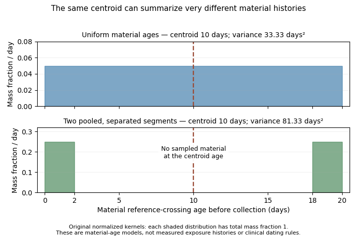
Two original material-age kernels have the same mean age but different spread and sampled intervals
. The lower kernel pools two separated segments of equal mass. Its mean age lies in a gap containing no sampled material. These are hypothetical reference-crossing ages, not observed exposure histories. Details.The centroid has a precise averaging property. For any representative time ,It minimizes the mass-weighted squared timing discrepancy. Also, if retained concentration is affine in , its kernel average equals its value at . This equality generally fails for a nonlinear history: a quadratic averages to , not .
A primary growth experiment followed marks near the proximal nail fold over measured intervals.[ref]
Growth rate of human fingernails and toenails in healthy American young adults by S. Yaemsiri and others. Abstract, Methods
Such displacement observations help constrain the material clock. They do not establish the full kernel, marker retention or one unique exposure date. Report the reference, distributional width and pooling assumptions alongside a centroid date.The input gate in long short-term memory controls how much proposed new information is written into the memory state of a long short-term memory recurrent neural network. In a common modern form,Here is the candidate memory update, is the input-gate vector, and means componentwise multiplication. The sigmoid function places each gate component between zero and one. The forget gate in long short-term memory separately controls the existing memory: suppressing a new write does not by itself erase stored information.[ref]
LSTM: A Search Space Odyssey by Klaus Greff and others. Section II, Figure 1: memory update and input-gate role; equations here omit peephole connections.
For a scalar example, let , , and . Then . Increasing only to gives : a larger gate admits more of the negative candidate. The gate is a multiplier, not an instruction that the memory must increase.
The proposed write and its admission are learned separately. An input may suggest a strong candidate while the gate learns that this timestep should be ignored. This selective writing was part of the original memory-cell strategy for protecting information across long delays, together with gated reading through the output gate in long short-term memory.[ref]
Long Short-Term Memory by Sepp Hochreiter and Jürgen Schmidhuber. Memory-cell construction and input/output gates protecting constant error flow.
The forget gate in long short-term memory controls retention of the previous memory state in a long short-term memory recurrent neural network. In a simplified modern update,Each component of multiplies the corresponding old memory component. Values near one retain it strongly; values near zero suppress it. The input gate in long short-term memory controls the separate new-write term.[ref]
LSTM: A Search Space Odyssey by Klaus Greff and others. Section II and Figure 1; simplified form here omits peepholes.
If a scalar gate stays at and the new-write term is zero, then after steps . The half-retention time isThis gives an interpretable timescale for a learned multiplicative gate. An exact no-write term is an illustrative condition; finite logistic sigmoid function outputs are strictly between zero and one, though the candidate can itself be zero.
The forget gate was added after the 1997 architecture. Felix A. Gers, Jürgen Schmidhuber and Fred Cummins introduced adaptive forgetting to handle continuing streams where a memory needs to be reset rather than preserved indefinitely. The direct memory-path derivative contains products of forget gates; the full recurrent derivative also includes dependencies through other states and gates.[ref]
Learning to Forget: Continual Prediction with LSTM by Felix A. Gers, Jürgen Schmidhuber and Fred Cummins. Abstract and adaptive forget-gate motivation for continual prediction.
The output gate in long short-term memory controls how much stored memory is exposed as the recurrent output of a long short-term memory network. In a common form,The memory is , the exposed state is , is a logistic sigmoid function, and is the hyperbolic tangent. The output gate in long short-term memory modulates the exposed state rather than directly multiplying the stored memory itself.[ref]
LSTM: A Search Space Odyssey by Klaus Greff and others. Section II, Figure 1: output activation and gate; simplified no-peephole equations.
For example, if , then . An output gate yields , whereas yields . Both cases can have the same current memory. A small exposed value therefore does not establish that the internal memory has been erased.
Selective exposure lets a network retain information until it becomes useful for a later prediction. The original architecture combined output gating with an input gate in long short-term memory to regulate access to persistent memory. Changing the exposed state may affect later gate decisions, so “does not directly erase” does not mean the output gate has no influence on future memory evolution.[ref]
Long Short-Term Memory by Sepp Hochreiter and Jürgen Schmidhuber. Memory-cell input/output gates and long-delay learning motivation.
An LSTM memory cell is the state-carrying unit of a long short-term memory recurrent neural network. It maintains an internal memory whose update is controlled by gates, while an exposed state communicates selected information to the rest of the network. The memory and exposed output are different quantities.[ref]
Long Short-Term Memory by Sepp Hochreiter and Jürgen Schmidhuber. Memory-cell construction and gated access to persistent state.
In a simplified modern form, omitting peepholes,The LSTM forget gate regulates retention, the LSTM input gate regulates the candidate write , and the LSTM output gate regulates exposure. The componentwise product allows different memory coordinates to make different decisions.[ref]
LSTM: A Search Space Odyssey by Klaus Greff and others. Section II and Figure 1; the displayed simplified variant omits the baseline's peephole connections.
For a scalar example, , , and give . If , the output is only . A small output can coexist with substantial stored state; it does not demonstrate memory erasure.
The additive state path was designed to help learning across long delays. The original 1997 architecture had input/output gating; adaptive forgetting was introduced later for continuing streams. Preserving a direct gradient path addresses an important learning difficulty but does not guarantee unlimited or perfectly reliable memory for every task.[ref]
Long Short-Term Memory by Sepp Hochreiter and Jürgen Schmidhuber. Constant error flow and delayed-dependency experiments.
[ref]Learning to Forget: Continual Prediction with LSTM by Felix A. Gers, Jürgen Schmidhuber and Fred Cummins. Adaptive forget gate and continual prediction.
A liquid-liquid tie line joins the compositions of two liquid phases that coexist at a specified temperature and pressure. Its endpoints describe the separate phases; an interior point describes an overall composition formed from suitable amounts of them. The liquid-liquid tie line therefore connects equilibrium chemistry with material balance rather than describing a spatial boundary between layers.
For a binary mixture, use component-B mole fractions , and overall fraction . If is the mole-based phase fraction in phase , conservation of component B gives the lever rule:The endpoints must be different and . For invented coexistence endpoints , and overall , the result is . In a -mole sample, the phases contain and moles; their component-B amounts are and moles, totaling . These mole amounts do not specify the two layer volumes.
A ternary liquid-liquid tie line obeys the same vector balance. For chosen endpoint vectors and , a phase fraction gives . Every component must give the same . A normalized composition vector need not lie on this particular line; normalization alone does not establish compatibility with the proposed endpoints.
The lever rule determines amounts after equilibrium endpoints have been established; it does not select those endpoints. They can come from measured phase compositions or a stable common-tangent construction for phase coexistence. Reliable experiments control temperature and sample purity, measure the separated compositions and distinguish genuine liquid-liquid equilibrium from other phase behavior. An IUPAC reference-system assessment specifically warns that turbidity can confuse liquid–liquid and solid–liquid transitions.[ref]
Reference Materials for Phase Equilibrium Studies. 1. Liquid-Liquid Equilibria by Ala Bazyleva and others. Introduction, pp.1–2: composition measurement, emulsions, solid–liquid discrimination and reference-system validation.
For exchanging neutral components at a common temperature and pressure, activity equality for coexisting liquids expresses liquid-liquid equilibrium as , provided both thermodynamic activities use the same standard state. The basic equilibrium condition is equality of chemical potentials; equality of numerical activities follows only after their references have been matched.
Write the definition of thermodynamic activity aswhere is the molar gas constant and is temperature. Subtraction at equilibrium givesThe ratio is one when the two standard chemical potentials are the same. IUPAC defines activity relative to the specified standard chemical potential and distinguishes pure-phase and solute reference conventions.[ref]
Quantities, Units and Symbols in Physical Chemistry by IUPAC. §2.11, pp.57,59; §2.11.1(iv), pp.61–62.
Mixing conventions can therefore produce unequal activities for physically coexisting phases. For instance, if one reference exceeds the other by , its corresponding activity is half as large at the same chemical potential. Standard-state activity conversion changes the numerical coordinate, not the physical driving force.Equal thermodynamic activities also need not mean equal mole fractions. With a common pure-liquid reference, , where is an activity coefficient. An original symmetric regular solution example makes this quantitative. Set the dimensionless interaction parameter to . The model has coexisting component-A mole fractions and , withThus and , whileComponent B satisfies the analogous equality by symmetry. The different compositions are compensated by different nonideal environments. These are chosen model values, not experimental compositions. As in liquid-liquid equilibrium, satisfying equalities must be supplemented by stability against competing phase arrangements.
Pinned article: Introduction to the OurBigBook Project
Welcome to the OurBigBook Project! Our goal is to create the perfect publishing platform for STEM subjects, and get university-level students to write the best free STEM tutorials ever.
Everyone is welcome to create an account and play with the site: ourbigbook.com/go/register. We belive that students themselves can write amazing tutorials, but teachers are welcome too. You can write about anything you want, it doesn't have to be STEM or even educational. Silly test content is very welcome and you won't be penalized in any way. Just keep it legal!
Intro to OurBigBook
. Source. We have two killer features:
- topics: topics group articles by different users with the same title, e.g. here is the topic for the "Fundamental Theorem of Calculus" ourbigbook.com/go/topic/fundamental-theorem-of-calculusArticles of different users are sorted by upvote within each article page. This feature is a bit like:
- a Wikipedia where each user can have their own version of each article
- a Q&A website like Stack Overflow, where multiple people can give their views on a given topic, and the best ones are sorted by upvote. Except you don't need to wait for someone to ask first, and any topic goes, no matter how narrow or broad
This feature makes it possible for readers to find better explanations of any topic created by other writers. And it allows writers to create an explanation in a place that readers might actually find it.
Figure 1. Screenshot of the "Derivative" topic page. View it live at: ourbigbook.com/go/topic/derivativeVideo 2. OurBigBook Web topics demo. Source. - local editing: you can store all your personal knowledge base content locally in a plaintext markup format that can be edited locally and published either:This way you can be sure that even if OurBigBook.com were to go down one day (which we have no plans to do as it is quite cheap to host!), your content will still be perfectly readable as a static site.
- to OurBigBook.com to get awesome multi-user features like topics and likes
- as HTML files to a static website, which you can host yourself for free on many external providers like GitHub Pages, and remain in full control

Figure 2. You can publish local OurBigBook lightweight markup files to either OurBigBook.com or as a static website.
Figure 3. Visual Studio Code extension installation.
Figure 5. . You can also edit articles on the Web editor without installing anything locally. Video 3. Edit locally and publish demo. Source. This shows editing OurBigBook Markup and publishing it using the Visual Studio Code extension. 
- Infinitely deep tables of contents:




All our software is open source and hosted at: github.com/ourbigbook/ourbigbook
Further documentation can be found at: docs.ourbigbook.com
Feel free to reach our to us for any help or suggestions: docs.ourbigbook.com/#contact