Topics (384k) Articles (398k) Users (410) Discussions (242) Comments (383) Files (13k) New article

A symmetric beam-radius perturbation for overlap branch selection compares two controlled settings of one Gaussian beam radius: and , with known . Under the centred, matched-wavefront curvature model of reciprocal size-ratio ambiguity in centred Gaussian overlap, writeThe hyperbolic secant form makes the symmetry explicit: the two settings evaluate the same even function at and . Their ordering identifies the sign of , as shown in branch selection by a controlled beam-radius change.
An original extension removes an unknown common scale and recovers the radius ratio itself. Suppose the two measured positive efficiencies satisfyThe factor is a shared multiplicative nuisance parameter, such as an unchanged response normalization. The symmetric log-overlap ratio eliminates it exactly:For the last equality, use the addition formula for hyperbolic cosine to write the fraction as , where . The defining logarithmic identity for the inverse hyperbolic tangent completes the derivation. Because , is positive for the initially narrower beam, negative for the wider beam, and zero at matching.
The inversion of a symmetric Gaussian overlap log-ratio now givesA finite radius ratio exists exactly when . This condition follows from ; equality is approached only as one radius ratio tends to zero or infinity. A measured log-ratio outside that interval has no finite solution in this ideal two-setting model.
For an original numerical example, take , true and unknown scale . The ideal readings are and . They give , recovering without supplying to the inversion. The physical bound is .
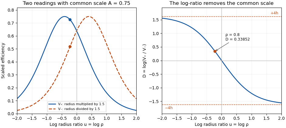
Two symmetric radius settings remove a shared scale and determine the signed Gaussian radius mismatch
. Original exact model with radius multiplier 1.5 and common efficiency scale 0.75. The left panel shows the two efficiency readings; the right shows their scale-independent log-ratio, its limiting bounds and the worked radius ratio 0.8. All curves are analytical model predictions. Details.Finite measurement noise still limits branch selection. For small relative errors, the delta method givesA perfectly shared multiplicative fluctuation cancels sample by sample, paralleling common-gain cancellation in heterodyne overlap uncertainty. Independent relative standard uncertainties of in the two readings instead give . At the worked point, the derivative of the inverse gives , hence about relative standard uncertainty in . At exact matching the two branches coincide; a noisy sign cannot identify a distinct physical branch there.
These conclusions require and the other optical mode matching conditions to remain shared across the settings. Changing a lens can alter wavefront curvature and polarization as well as radius. NIST's physical heterodyne apparatus explicitly controlled polarization and spatial matching.[ref]
Frequency response metrology for high-speed optical receivers by Paul D. Hale and others. PDF p. 1, Heterodyne measurements
Larger radius changes may strengthen the log-ratio response while lowering either measured efficiency and changing its noise. Step choice therefore depends on the apparatus and noise model.A bearing axial tolerance stack expresses the effect of contributing dimensional deviations on the realized axial position of a bearing assembly. Each contribution enters with the sign and sensitivity imposed by the geometry. The resulting setting variation consumes bearing axial travel margin. The manufacturer's locating/non-locating bearing discussion identifies relative axial displacement and accumulated dimensional variation as design considerations.[ref]
Rolling bearings by SKF. Section B.2, printed p.70, relative displacement and tolerance accumulation
For an original linear stack, let shaft, housing and shim deviations be , and , with setting errorIf their independent admissible ranges are respectively , and , the worst-case setting range is . The positive extreme uses the upper shaft and shim deviations with the lower housing deviation. Here “independent admissible ranges” means that all combinations are allowed, rather than a probabilistic independence assertion.
A design with nominal margin0.10mm and required reserve0.05mm can accommodate at most0.05mm of bounded setting error. This stack is therefore too wide by0.01mm. Reducing the housing deviation bound from0.03 to0.02mm makes the worst-case sum0.05mm and meets that geometric reserve exactly. A bearing nominal axial setting can shift the range but cannot shrink its width.
Statistical propagation answers another question. With coefficient vector and covariance matrix , the setting variance isFor independent errors with standard uncertainties0.010,0.010 and0.005mm, this gives . If the shaft and housing errors instead have correlation0.9 while the shim remains independent, the subtraction cancels much of their shared variation:giving about0.00671mm. Reversing a geometric sign or changing correlation changes that result. The GUM requires the covariance contribution when inputs are correlated.[ref]
Guide to the expression of uncertainty in measurement by JCGM. §5.2.2, equation13, correlated-input uncertainty
Neither statistical value replaces the0.06mm deterministic bound without a justified model relating probabilities and allowed ranges. Shared reference measurements or common thermal conditions can introduce dependence. Keeping the dimensional signs, bounds and covariance assumptions in the stack makes the resulting bearing axial setting tolerance reproducible.
Conditioning of two-span beam compliance inference describes how perturbations in two measured compliances and support spans affect the inferred bending coefficient. In the model represents an unchanged series contribution and is beam flexural rigidity. The cubic beam term follows from the midspan compliance of a simply supported beam.[ref] The subtraction is sensitive when the spans are close, or when the beam-response difference is small compared with readout errors.
Let and temporarily treat the spans as exact. The sensitivity coefficients are and . Consequently,This is the standard measurement uncertainty propagation rule applied to a linear combination; the covariance term matters when the readings share errors.[ref]
For an original numerical comparison, stipulate , so , and independent standard uncertainties . Spans and give and , about 54 percent of . Increasing the second span to gives and , about 3.57 percent. The wider spacing makes the same compliance readout precision much more informative.
Span uncertainty enters through additional sensitivity coefficients:For uncorrelated span readings, their first-order contribution to is , before any compliance/span correlations are included. An identical additive readout offset cancels from , whereas a changing offset does not.
A practical span comparison holds the specimen, contacts, loading position and displacement channel as consistent as possible. Close spans amplify measurement noise; simply choosing distant spans can instead expose a failure of the assumed model. Shear produces a term proportional to , and changing contacts can change . A third span tests those assumptions. Finally, inversion to is strongly nonlinear near : the 54-percent case cannot be adequately summarized by a small symmetric relative uncertainty on .
The volt-ampere, symbolVA, is the unit commonly used to express apparent power. At a terminal pair, RMS potential difference in volts multiplied by RMS current in amperes gives the numerical value in volt-amperes. The unit product has the same coherent SI dimensions as the watt:This unit identity does not make apparent power and active power the same quantity. The SI text explicitly warns that different physical quantities can share a unit and that the quantity must be specified.[ref]
The International System of Units (SI), ninth edition, SI Brochure. NIST SP330 parallel text, §2.3.4, coherent derived units and quantity identification
For an original example,250V RMS at8A RMS gives2000VA, or2kVA. If the absorbing load has power factor0.75, its active power is1500W. A1500W value cannot be inferred from the2kVA alone without the phase/waveform information summarized by that factor.
Hypothetical equipment can have separate apparent- and active-power limits. A1000VA/600W limit would permit a500W, factor0.5 load only at the apparent-power boundary, since it requires1000VA. A700W, factor-one load would require only700VA but exceed the separate600W limit. These examples interpret stated numerical constraints rather than specify an actual product's behavior.
For single-frequency sinusoids, the magnitude of complex electrical power is expressed in volt-amperes, while its real part is commonly expressed in watts and its imaginary part in reactive volt-amperes. Those names help keep the quantities distinct even though their base-unit dimensions agree.[ref]
AC Power Flow in Linear Networks by James L. Kirtley Jr.. Energy and Power, equations61–63; §7.1 RMS Amplitude
With distorted signals, retain the actual RMS-product definition of apparent power rather than assuming a single fundamental phasor accounts for all current.The category of affine schemes has affine schemes as objects and morphisms of schemes as arrows. The contravariant functor gives an equivalencewith the opposite of the category of commutative rings. Precisely, every ring homomorphism corresponds to a unique map , and every morphism of schemes between affine schemes arises this way.[ref]
For example, , , induces the squaring map of affine lines. A map from to instead corresponds to a -algebra map , expressing a rational point. A Cartesian product of affine -schemes corresponds to a tensor product of commutative algebras: . Reversing arrows explains why geometric products become algebraic coproducts.
Standard-state activity conversion changes the numerical thermodynamic activity assigned to a fixed physical state when its reference chemical potential changes. The observable equilibrium and physical chemical potential stay the same. The activity and its standard chemical potential must therefore be converted together.
At fixed temperature , writeIf , subtraction givesHere is the molar gas constant. This follows from the IUPAC definition of relative activity and its specified standard state.[ref]
Quantities, Units and Symbols in Physical Chemistry by IUPAC. §2.11, pp.57,59, and §2.11.1(iv), pp.61–62: activity and reference conventions.
Changing just the activity in the first equation would instead change the calculated physical chemical potential.For an invented conversion , the compensating reference shift is . An old activity becomes ; the two expressions for are identical. An activity of one consequently identifies a reference condition under the chosen convention, not an invariant amount of material.
An activity conversion of an equilibrium constant follows the same logic. For the reaction A B, take at equilibrium and convert by , . Then . If , the converted value is , whilebecause originally . For any physical composition, the corresponding reaction quotient also changes by , so remains unchanged. These are reference changes, not altered reaction chemistry.
The same requirement governs activity equality for coexisting liquids: compare activities only after identifying their standard states, composition scales and reference conventions. Equal numerical values expressed under incompatible conventions do not, by themselves, establish liquid-liquid equilibrium.
Two-state vibrational frequency memory models a probe that switches between two frequency environments while retaining a time-dependent relation to its earlier state. It distinguishes state occupancy, a vibrational frequency-state residence time and decay of the vibrational frequency-frequency correlation function.
Let a continuous-time Markov chain switch from state A to B at rate and from B to A at rate . Its stationary probabilities areFor spectroscopic wavenumbers , the stationary mean is and the variance isThe centered state values form a decaying mode of the two-state transition generator, with rate . Consequently,The vibrational frequency-state residence times are instead in A and in B. Correlation decay includes paths that leave and return, so it is not identical to survival without a switch.
Starting in A, the probability of being in A later isAt it is about , while the probability of never leaving A is only . Their difference includes return trajectories. At long times, the stationary probability of matching the initial state approaches , while normalized frequency covariance tends to zero. A nonzero same-state baseline therefore need not mean persistent covariance.
Primary two-dimensional infrared spectroscopy theory connects waiting-time-dependent spectral geometry with frequency memory under response approximations.[ref]
Frequency-frequency correlation functions and apodization in two-dimensional infrared vibrational echo spectroscopy: A new approach by Kyungwon Kwak and others. Introduction and Section II.A, frequency labeling and correlation-function description
The rates and wavenumbers above are illustrative. A real assignment also needs spectral resolution, pulse characterization and a population-relaxation model; agreement with one exponential decay does not uniquely establish two microscopic states.Common-gain cancellation in heterodyne overlap uncertainty is the exact invariance of the normalized beat amplitudewhen the corrected peak beat current and both separately measured arm currents are multiplied by the same factor . The factor occurs once in the numerator and once in the denominator. This is scale invariance: the ratio is a homogeneous function of degree zero. The cancellation holds for every realization of a random common factor, without requiring it to be independent of the currents.
More generally, take and let their residual multiplicative measurement calibration factors be . The observed normalization satisfiesThus the gain-matching condition for heterodyne normalization is ; the three factors need not all be equal. For example, , and leave the ratio unchanged. The denominator depends on the geometric mean of its two factors.
Writing the natural logarithms of the factors as a random vector makes the remaining uncertainty particularly clear. With ,This identity is exact for the logarithmic error. The relative variance of the original ratio is only approximately equal to it when the errors are small, as in the variance of a corrected heterodyne overlap estimate. Keeping the covariance terms follows the general measurement-propagation rule.[ref]
For an original imperfect-sharing model, set . Assume are zero-mean independent random variables. The coefficient of the shared fluctuation is , soTake , , with standard deviations for , for and for each arm's separate error. Then and , giving logarithmic standard uncertainty , approximately relative uncertainty. A large shared fluctuation can leave a small residual, but incomplete matching prevents exact cancellation.
If the log-errors additionally have a normal distribution, then and the normalized readout has a lognormal distribution. Its exact expected value is , not . At , this example gives mean and standard deviation . The lognormal bias of a heterodyne overlap estimate comes from exponentiating the remaining error; the perfectly shared factor still cancels.
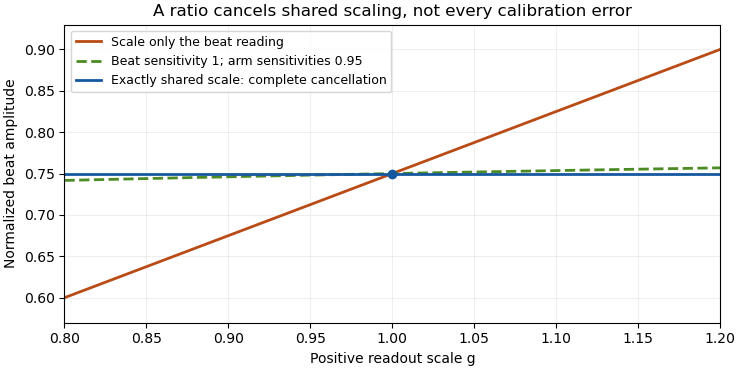
The physical calibration paths determine which model applies. NIST's receiver experiment combined two lasers through a beam splitter, polarizer and single-mode optical fiber, while separately correcting electrical loss and impedance mismatch.[ref]
Frequency response metrology for high-speed optical receivers by Paul D. Hale and others. PDF pp. 1–2, Heterodyne measurements and equations 1–4
An electronic gain change confined to the beat-frequency path need not appear in the arm-current measurements. Likewise, adding a current offset is not multiplication by a common factor. Background correction and the sharing of calibration factors must therefore be established before claiming cancellation.Character-device lifetime after deletion is the interval during which a removed character device still needs valid backing state because existing users can invoke its operations. Linux
cdev_del removes the device from new-open lookup; it does not invalidate already-open file descriptors. The kernel explicitly permits their file-operation callbacks after deletion returns.[ref]Character-device number registration in the Linux kernel documentation. Char devices, cdev_del lifetime note
Consider an original event sequence. Process A opens an interface and retains a pointer to driver state. Removal calls
cdev_del; process B can no longer obtain a new open through that registration. Process A then calls read. Freeing the state immediately after deletion would make that callback access dead storage: a use-after-free. The lookup lifetime and the backing allocation lifetime are different.A useful ownership model gives the allocation one registration reference and one reference for each successful open. In a simplified reference counting design with opens, the reference count is . Removal drops the registration reference; each final close drops its open reference. With two opens, the sequence is , and storage is reclaimed only at zero. This is a model of ownership, not a complete driver implementation: taking references must itself be synchronized with removal, and asynchronous work can require additional references.
The character device may be disconnected from its hardware before its storage is reclaimed. Existing operations can observe a synchronized disconnected state and return an appropriate error while the allocation remains valid. Reference protection alone does not make removed hardware usable or serialize simultaneous operations.
For combined device objects,
cdev_device_add and cdev_device_del have their own documented pairing and parent-reference rules. The add helper can expose callbacks even when it reports failure; the delete helper distinguishes stopped sysfs callbacks from still-callable operations on existing opens.[ref]Character-device number registration in the Linux kernel documentation. cdev_device_add description and failure warning; cdev_device_del note
Therefore unwinding a failed character-device registration must follow the actual publication and ownership state. Releasing the device number reservation is separate from proving that every user of private storage has finished.Extremal calibration for nested confidence families obtains simultaneous protection for many candidate bounds by checking their most demanding marginal endpoints. It uses the ordering of a nested family rather than treating every candidate as an unrelated comparison. The simultaneous event then also protects a choice made after observing the data.
Consider the detection model , with upper confidence bounds decreasing in their failure budget and lower bounds increasing in . For a prescribed set of candidate allocations , let and be the largest respective budgets, with valid bounds defined at those endpoints. Onevery candidate satisfiesThe union bound gives simultaneous coverage at least . Neither independence of the estimates nor a finite number of candidates is needed for this common-event proof.
For the line segment , , the endpoints are and . The protected failure budget is therefore . The width of the candidate interval consumes part of the simultaneous budget; it cannot be ignored simply because every point on the segment has the same marginal budget sum.
An original exact-tail example has zero detections in and successful detection of all measurement calibration positives. Binomial distribution tail inversion gives and . NIST describes the one-sided tail construction and simultaneous error-budget principle.[ref]
NIST and SEMATECH e-Handbook of Statistical Methods. §7.2.4.1, exact one-sided intervals; §7.4.7.3, Bonferroni's method
For candidates and , the bounds are about 0.13946 and 0.12201. Their extremal endpoint combination gives about 0.11956 and at least 95% coverage. It is a tighter bound with the larger combined budget, and its validity follows directly from the endpoint event.The construction requires the stated nesting and valid endpoint bounds. A family whose order reverses or whose measurement calibration changes across candidates needs a new argument. If the lower endpoint bound for detection is zero, the prevalence upper bound is one, rather than an undefined division.
Bootstrap ratio bias with unequal cluster sizes arises because the pooled mean in a cluster bootstrap is a ratio with a random denominator. Let the empirical distribution over the observed groups assign mass to each pair of group size and response sum. One bootstrap replicate draws such pairs and computes . Its conditional expectation need not equal , even though the numerator and denominator averages are individually unbiased for their empirical means.
A second-order Taylor expansion of explains the leading effect. Write and for the empirical variance of one group size and empirical covariance of one group size with its response sum, using denominator . The conditional bootstrap bias is approximatelyThe second derivatives are and ; the variances/covariance of the averages bring in . This delta method approximation requires a denominator sufficiently concentrated away from zero and control of the remainder. It is not an exact identity for a few highly unequal groups.
For an original three-group example, take . Then , , , and . The second-order bias estimate is . Enumerating all ordered bootstrap draws instead gives mean about , hence exact conditional bias about . The approximation identifies the direction and mechanism but misses a visible remainder at this small group count.
Equal group sizes remove the random denominator and this particular ratio bias. If every group has the same response mean, , every replicate ratio is exactly regardless of size. Neither case justifies replacing a row-weighted estimand with an equally weighted group mean in general; see unequal-cluster weighting in a cluster bootstrap. The primary Stata specification samples entire clusters and allows replicate row counts to vary.[ref]
Bootstrap sampling and estimation in the Stata documentation. Printed pp. 3–5, cluster() and variable replicate size
Pivot-location uncertainty in a rotational clearance bound describes how an error in the point about which a rigid rotation is modeled changes predicted occupied-point motion. A radius measured about one pivot is not automatically valid about another. The underlying planning problem must include both translation and orientation of the robot’s actual geometry.[ref]
Robotic Systems by Kris Hauser. Chapter 9, C-obstacles for rotational motion and Motion planning in SE(2)
Let be a fixed rotation matrix, the modeled pivot, and the actual pivot. First suppose the initial physical point is known exactly and both descriptions use the same rotation . The modeled and actual endpoints areso their difference is exactlyThis vanishes for zero rotation even if the pivot location is uncertain. Treating pivot error as an arbitrary full translation at every angle can therefore be unnecessarily conservative.
For a rotation through principal angle about a known axis direction, the component of along that direction is unchanged by . Its perpendicular component giveswhen . The chord-length factor is the same geometry used in the angular clearance bound for a rotating body. For a rotation and , the maximum endpoint error from pivot location alone is about . An equally large pivot offset parallel to the axis produces no endpoint change in this model.
If the initial point also has error with , thenFor the difference of displacement vectors, rather than final positions, the shape term is , giving the different bound . The requested geometric quantity determines which allowance applies.
A complementary radius argument bounds total actual motion. If modeled points satisfy , then , and total point displacement is at most . This is the enclosure approach in uncertainty in a rigid-body bounding radius; it need not equal an endpoint-error calculation against a nominal path.
Correlations can reduce the bound. If the same coordinate-frame translation shifts both the modeled point and pivot, relative geometry may be unchanged; treating those two descriptions as independent physical errors loses that cancellation. Conversely, rotation-axis direction uncertainty in clearance bounds changes itself and is not covered by the fixed- pivot formula.
A proposed rotary-stage check observes several rigid fiducials, estimates the pivot and axis in one coordinate frame, and compares independent endpoint measurements at several angles with the predicted chord scaling. Include attached tools and measurement uncertainty. When the robot moves against an uncertain obstacle, combine this occupied-point model with a separately justified distance-query enclosure; a correct pivot bound does not establish the obstacle model’s accuracy.
Section compression is shortening of a cut section relative to the corresponding specimen-block dimension, usually measured parallel to the cutting direction in ultramicrotomy. It is a physical deformation introduced during preparation, so an accurately calibrated microscope can still measure a distorted specimen. Manufacturer guidance for polymer sectioning connects reduced compression with smaller knife wedge angles, while noting the resulting greater sensitivity of the cutting edge.[ref]
Ultramicrotomy Techniques for Materials Sectioning by Leica Microsystems. How to prepare high-quality sections of polymers: wedge-angle tradeoff
Let be a reference length in the block and its recovered section length along the same direction. Define a positive compression fractionThe corresponding engineering strain is . State this sign convention: a reported positive percentage compression and a negative longitudinal strain can describe the same shortening.
For an original geometrical model, a feature recovered as has . If transverse dimensions are unchanged and the shortening is uniform, an originally circular feature becomes an ellipse with axis ratio . Its area becomes of the original, not : only one direction was shortened. Under the additional assumption of volume conservation, a nominal layer would have thicknessNeither transverse constancy nor volume conservation is automatic. Material loss, cracking, relaxation and nonuniform deformation can invalidate the model; section length alone cannot establish recovered thickness.
A useful materials check compares recognizable features in the block face and collected section, recording cutting direction, knife wedge angle, knife clearance angle and specimen conditions. Repeating the comparison at several positions tests whether one compression fraction is adequate. Under the simple model above, expanding the shortened coordinate by would reverse the geometrical shortening, but this is a model-based correction rather than an extra observation. Image registration can align features without proving that it has recovered their original shapes.
A right-topological semigroup is a semigroup with a topology such that, for each fixed , the right translation is a continuous map. The varying input is on the left. Requiring instead gives a left-topological semigroup; requiring multiplication jointly continuous gives a topological semigroup.
For a one-sided example, take all functions with function composition and the product topology, so convergence is pointwise convergence. For fixed , the map is continuous because its value at is the evaluation of at the fixed point .
Left composition can fail to be continuous. Let for and zero otherwise, and let be constant . Then converges pointwise to the zero function, but is constantly one while is constantly zero. Thus right-translation continuity alone does not imply continuity of the other translations.
The tidal range is the difference in sea-surface height between a specified high tide and the neighboring low tide, measured relative to the same datum. A high-water level of and low-water level of give a range of .
For a sinusoidal tide , the range is , not the amplitude . Interference between lunar and solar tidal contributions produces larger spring ranges and smaller neap ranges. Coastline geometry, water depth and resonance modify the local response, so the tidal range cannot be inferred from astronomical forcing alone.
A ghost-level consistency test for a delayed pulse replica checks whether measured side lobes agree with the simple model of one real delayed pulse and its nonlinear correlation ghost. It can reject that model; agreement alone does not prove that no real prepulse exists.
Use the separated, identical-shape replica model in third-order pulse correlation ghost. Let be the positive-delay lobe and the opposite-delay lobe, each divided by the central correlation peak. For delayed-to-main intensity ratio ,Thus the measured ratio gives , and the first equation supplies an additional consistency condition. The frequently useful approximation omits the small central-peak correction; exactly, .
For an original pair of measured relative heights and , their ratio would require . That value predicts , not . These two readings therefore cannot both come from the stated single-replica model with equal instrument sensitivity at the two delays. A real earlier pulse is one possible explanation, but background, unequal pulse shapes or additional replicas can also invalidate the model.
An independent check varies the delayed replica while holding the main pulse fixed. Before central-peak normalization, halving halves the real side lobe and quarters its ghost. This attenuation scaling of a third-order correlation ghost probes the nonlinear origin rather than only one accidental height match. The existing parent diagram shows a direct numerical example without an actual pulse at the ghost's delay.
The historical correlator's inserted-etalon experiment provided a controlled physical postpulse and a known temporal direction.[ref]
A Single Shot 3rd Order Cross-Correlator for Pulse Contrast and Pulse Shape Measurements by J. Collier and others. printed p. 195, Results and Figure 4
The algebraic height test here is an independent ideal calculation. Use unsaturated, background-corrected readings with comparable response and lobe resolution; otherwise the measured ratios need not represent the model's intensities.Gaussian instrument broadening in third-order pulse correlation is the widening produced when an ideal third-order intensity autocorrelation is convolved with an additional Gaussian instrument response. It is a model of the measurement, not a universal correction for every correlator. The finite width of the optical nonlinear gate is already part of the ideal third-order trace and must not be counted again as an independent response.
Let a Gaussian pulse have intensity standard deviation . Its ideal trace is a Gaussian with . Take the additional normalized impulse response to beThe convolution isThe response preserves integrated trace area while reducing peak height and increasing variance. Since every Gaussian full width at half maximum has the same conversion factor from standard deviation,
For an original example, and give an ideal correlation width about and a measured width about . The peak falls to approximately 0.853 of the ideal peak under this unit-area response. Dividing the measured width only by would overestimate the pulse duration.
The correct Gaussian inversion is when the radicand is positive. Its conditioning worsens near the response floor: the derivatives with respect to and are and . Small width errors can therefore cause large errors in a narrowly resolved pulse. Gaussian pulse-width deconvolution uncertainty must include uncertainty of the characterized response, with covariance if relevant.
The primary correlator used second-harmonic generation, sum-frequency generation, crossed beams and spatial imaging to encode delay. It did not assert that every additional broadening mechanism was a Gaussian convolution.[ref]
A Single Shot 3rd Order Cross-Correlator for Pulse Contrast and Pulse Shape Measurements by J. Collier and others. printed pp. 194–195, third-order integral, Description and Figure 2
To apply this model, characterize the response under the same optical alignment, spectral acceptance and detector conditions. Non-Gaussian wings, clipping or unresolved side lobes require a different model; a smaller sampling step cannot by itself remove optical broadening. Pinned article: Introduction to the OurBigBook Project
Welcome to the OurBigBook Project! Our goal is to create the perfect publishing platform for STEM subjects, and get university-level students to write the best free STEM tutorials ever.
Everyone is welcome to create an account and play with the site: ourbigbook.com/go/register. We belive that students themselves can write amazing tutorials, but teachers are welcome too. You can write about anything you want, it doesn't have to be STEM or even educational. Silly test content is very welcome and you won't be penalized in any way. Just keep it legal!
Intro to OurBigBook
. Source. We have two killer features:
- topics: topics group articles by different users with the same title, e.g. here is the topic for the "Fundamental Theorem of Calculus" ourbigbook.com/go/topic/fundamental-theorem-of-calculusArticles of different users are sorted by upvote within each article page. This feature is a bit like:
- a Wikipedia where each user can have their own version of each article
- a Q&A website like Stack Overflow, where multiple people can give their views on a given topic, and the best ones are sorted by upvote. Except you don't need to wait for someone to ask first, and any topic goes, no matter how narrow or broad
This feature makes it possible for readers to find better explanations of any topic created by other writers. And it allows writers to create an explanation in a place that readers might actually find it.
Figure 1. Screenshot of the "Derivative" topic page. View it live at: ourbigbook.com/go/topic/derivativeVideo 2. OurBigBook Web topics demo. Source. - local editing: you can store all your personal knowledge base content locally in a plaintext markup format that can be edited locally and published either:This way you can be sure that even if OurBigBook.com were to go down one day (which we have no plans to do as it is quite cheap to host!), your content will still be perfectly readable as a static site.
- to OurBigBook.com to get awesome multi-user features like topics and likes
- as HTML files to a static website, which you can host yourself for free on many external providers like GitHub Pages, and remain in full control

Figure 2. You can publish local OurBigBook lightweight markup files to either OurBigBook.com or as a static website.
Figure 3. Visual Studio Code extension installation.
Figure 5. . You can also edit articles on the Web editor without installing anything locally. Video 3. Edit locally and publish demo. Source. This shows editing OurBigBook Markup and publishing it using the Visual Studio Code extension. 
- Infinitely deep tables of contents:




All our software is open source and hosted at: github.com/ourbigbook/ourbigbook
Further documentation can be found at: docs.ourbigbook.com
Feel free to reach our to us for any help or suggestions: docs.ourbigbook.com/#contact