Topics (384k) Articles (398k) Users (410) Discussions (242) Comments (383) Files (13k) New article

Contact-mode numerical phase error is the difference between the oscillation phase produced by a time integrator and the phase of the modeled contact dynamics. It can grow while the numerical solution remains bounded. Contact-mode timestep stability controls a different property; stable integration alone does not ensure accurate force timing or contact-event timing. The physical motivation is the fast oscillation introduced by a stiff compliant contact model.[ref]
Underactuated Robotics by Russ Tedrake. Multi-Body Dynamics, Compliant Contact Models, stiff-spring and numerical integration discussion
For a frozen undamped contact mode , central differences givePut and use . On the stable branch ,The numerical frequency exceeds the modeled frequency. A Taylor series givesFor the trapezoidal rule, its amplification-factor phase instead givesThat scheme preserves modal amplitude in this undamped linear setting while lagging in phase. These formulas isolate a single mode with fixed frequency and consistent initialization; general nonlinear contacts require additional analysis.
Accumulated contact-mode phase drift after a duration is at time-grid points. For an original example, let and . With , the central-difference frequency is about , producing of phase lead. The step satisfies the strict stability inequality, yet the phase lead exceeds half a cycle.
Reducing to gives about of lead over the same duration. At it is about , approximately one quarter as large, matching the leading second-order error. For a small desired phase budget , the central-difference expansion suggestsWith , this estimate is about , much smaller than the stability boundary. Check the exact frequency formula when the small-step expansion is not sufficiently accurate.
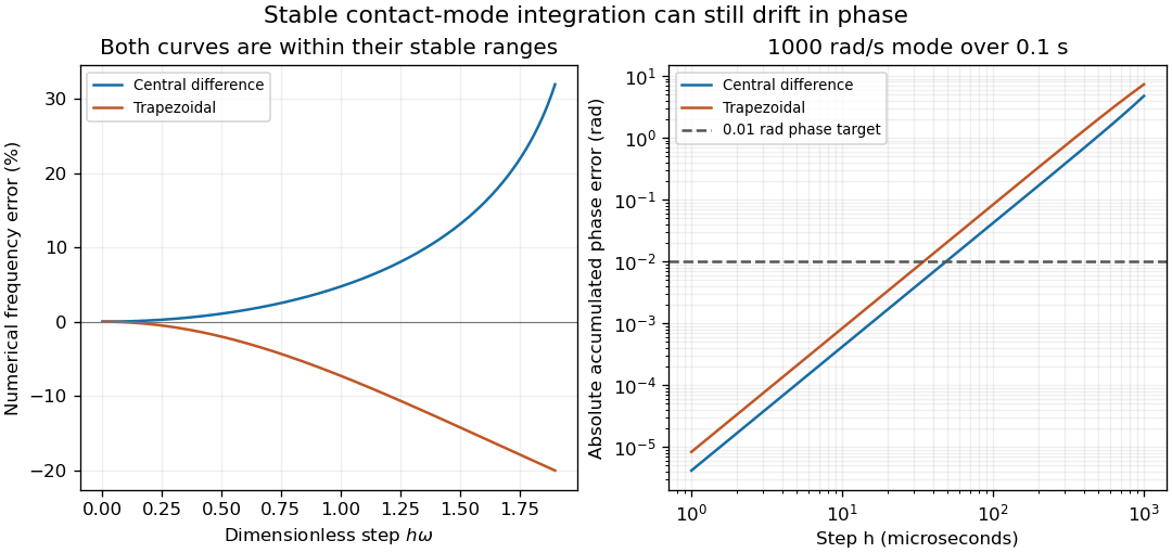
Stable contact-mode timesteps can accumulate substantial numerical phase error
. Exact frequency errors for central differences and the trapezoidal rule, and the resulting absolute phase errors for a fixed 1000 rad/s mode integrated over 0.1 s. The horizontal line is an illustrative 0.01 rad phase budget. These are analytical linear-mode predictions, not contact measurements. Details.In a contact experiment or simulation, a shifted oscillation phase changes when force maxima and gap crossings are predicted. Damping, changing tangent stiffness and a contact opening can invalidate the fixed-frequency model, so the phase estimate is not by itself an event-time error certificate. A proposed convergence check compares force histories, dominant frequency and event times at successively halved steps, while keeping contact geometry and constitutive parameters fixed. Agreement in maximum penetration alone can miss a phase error that accumulates over many cycles.
Compatibility of bounded endpoint distance queries asks whether two uncertain distance readings could arise from any nonnegative clearance function obeying a stated motion bound. It tests consistency of the observations and assumptions; it does not itself prove that the entire motion is collision-free.
Suppose endpoint queries yield intervals and for the true set distances, with . Let the interval duration be and clearance have Lipschitz continuity constant . Write . Compatibility means there exist and satisfying . The exact condition isalong with the two intervals being nonempty and nonnegative. Equivalently, the gap between the two intervals, , must not exceed .
Necessity follows because , and , with the reversed argument for the other inequality. For sufficiency, overlapping intervals allow at any common point. If they are disjoint, choose their nearest endpoints; the boxed condition bounds that separation by . Linear interpolation between the selected nonnegative endpoints has slope at most , proving that at least one admissible continuous clearance function exists.
The feasible endpoint intervals can be tightened toThese are the exact projections of the feasible endpoint-pair set onto each coordinate. A large difference between the lower bounds alone is not a contradiction: lower bounds are not exact distances.
For an original example, take , and . Their nearest endpoints differ by , so the data are compatible. Tightening gives and . By contrast, and have a minimum gap and are incompatible with the same motion bound.
Incompatibility means that some query enclosure, motion bound, timing or model assumption is wrong. It is not evidence that a collision occurred. Compatibility also need not certify separation: exact endpoint distances of over one second with permit both constant clearance and a V-shaped clearance touching zero halfway through. The clearance certificate with bounded distance-query error evaluates a lower envelope over the full interval to answer that additional question.
For , compatibility reduces to overlap of the intervals because clearance is constant. With more query times, multi-sample consistency of distance-query intervals must preserve one common clearance model rather than checking unrelated pairs with incompatible bounds. The primary motion-planning formulation requires constraints along a continuous path, motivating these between-sample checks.[ref]
Robotic Systems by Kris Hauser. Chapter 8, Point-to-point path planning; Chapter 9, configuration-space obstacles
A proposed checker retains query lower and upper bounds, the clock interval, geometry version and motion allowance. It should report inconsistent inputs separately from undecided clearance intervals and certified margin violations. Tight numerical arithmetic alone cannot turn an unsupported standard uncertainty into a deterministic distance enclosure.
A centripetal speed-gain error is an error in a calculated centripetal correction caused by a multiplicative scale error in the measured angular velocity. For true centripetal magnitude and indicated speed , the computed magnitude with correct radius isWriting gives exact relative error . The leading relative error is therefore twice the speed-scale error, rather than equal to it.
For an original example, let and , giving . A1% high speed indication gives , an overestimate4.02m/s². Subtracting that value from a radial reading would leave an error of the opposite sign if the true motion were otherwise modeled correctly. The example illustrates sensitivity; it is not a measured calibration error of a particular sensor.
Radius error combines with speed gain. If the indicated radius is , thenTo first order, relative error is . Apparent cancellation between these terms at one condition does not separately identify either calibration parameter. An independent radius measurement or speed reference helps distinguish their contributions.
An additive speed offset behaves differently:Measurements at several speeds can distinguish the quadratic scale contribution from the linear and constant offset contributions, subject to the remaining model and measurement errors. Near zero true speed, a relative-error description becomes unsuitable even though the absolute expression remains meaningful.
The same gain factor applies to the first-order ripple correction when both mean speed and ripple amplitude share that speed scale. The resulting mismatch enters the centripetal amplitude-error budget, while relative channel timing enters the centripetal phase-error tolerance. A primary rotating MEMS-sensor experiment identifies rotating-frame components and reconstructs a rotation reference, making the physical need for consistent speed and timing information concrete.[ref]
Evaluation of MEMS-Based Wireless Accelerometer Sensors in Detecting Gear Tooth Faults in Helicopter Transmissions by David G. Lewicki and others. Printed pp.19–21, rotating-frame components; pp.24–25, timing reconstruction
At a specified operating point, the sensitivity coefficient to speed is . A speed standard uncertainty therefore contributes approximately to the correction's standard uncertainty, with radius uncertainty and any covariance included separately.[ref]
Guide to the expression of uncertainty in measurement by JCGM. §5.1.3 and §5.2, sensitivity coefficients and correlated inputs
An exponential-envelope tail-energy bound limits unobserved energy by integrating a justified pointwise envelope on the true optical power. If for every , with and , then . The parent bounding unobserved optical energy with an exponential tail model derives this result and distinguishes it from a statistical uncertainty.
At a later acquisition endpoint , the remaining allowance isFor an original envelope with and , the initial allowance is . Reducing the allowed missing energy to requires . This acquisition duration from an exponential tail-energy tolerance reduces the bound by a factor100. It does not prove that99% of an arbitrary underlying pulse has been captured: the actual power may lie strictly below the envelope at early times.
Joint parameter constraints also matter. An original allowed set uses dimensionless and with , and . Since , every allowed envelope satisfiesattained at . Taking separate maxima and would instead give the looser bound; those two maxima cannot occur together in the stated joint set.
The guarantee concerns optical power, not an uncorrected detector tail. Optical tail and detector-response ambiguity explains that distinction, while NIST's primary response-calibration procedure characterizes the electrical measurement chain separately.[ref]
Calibration Service for Low-level Pulsed-Laser Radiometers at 1.06 µm: Pulse Energy and Peak Power by Rodney W. Leonhardt. Appendix C.1–C.2, printed pp. 36–37
A delayed extra pulse or an unbounded constant background requires its own model; neither is excluded by a local exponential fit.Optical tail and detector-response ambiguity arises because a measured temporal trace combines the optical waveform with the receiver's dynamics. In a calibrated linear time-invariant system,where is incident radiant power and the unit-area detector impulse response. One trace does not generally identify both unknown functions. The parent bounding unobserved optical energy with an exponential tail model gives an impulsive-input example; two finite-width profiles provide another exact ambiguity.
Define for , and zero otherwise. Consider model A with optical power and detector response , and model B with these two time constants exchanged. By commutativity of convolution, both give exactlyTheir optical energies after are nevertheless and . For original chosen , those are about and . Identical recorded tails therefore coexist with very different true late optical energy.
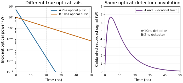
Different optical tails and detector responses can produce the same measured pulse
. Original unit-area exponential response models. Model A has a2ns optical time constant and10ns detector time constant; model B exchanges them. Both incident pulses have100nJ total energy. The measured convolution is identical despite different optical energy after20ns. Source. Details.Known-input calibration of a pulse detector supplies information missing from this inverse problem. NIST measured the detector/cable/oscilloscope response with optical excitation much shorter than the response before calculating waveform distortions.[ref]
Calibration Service for Low-level Pulsed-Laser Radiometers at 1.06 µm: Pulse Energy and Peak Power by Rodney W. Leonhardt. Appendix C.1–C.2, printed pp. 36–37, Figure C1 and bandwidth-correction procedure
The example above is an independent mathematical construction. A fitted electrical decay constant alone cannot establish a global optical-tail envelope.Capacitor-stage quantization error is the residual reactive power caused by choosing among discrete settings of a capacitor bank instead of a continuously adjustable correction. In a fixed sinusoidal operating model, let the load absorb and let the target residual be . The desired capacitive correction is . Selecting available correction leavesThe error concerns the selected setting, separately from sensing error, changing load and component tolerance.
For equal stages of magnitude and an available range covering the desired correction, nearest-stage selection chooses an integer nearest . HenceAt a half-stage tie either neighbor attains the bound. A policy forbidding a negative residual relative to zero instead rounds downward and gives , away from the bank's capacity limits. The two policies solve different constrained problems.
For an original zero-target example, let and . Three stages give ; two give . With active power , nearest-stage selection guaranteesprovided the zero-reactive target is within range and the sinusoidal fixed-load assumptions hold. At only , the same worst-case bound falls to about . A stage size suitable at high demand need not give the same numerical power factor at low demand.
Unequal stages require the actual attainable set. Stages of 100 and 400 vars permit vars. At a desired 250 vars, the nearest setting leaves 150 vars error, despite the smallest stage being only 100 vars. The relevant bound is half the largest gap between neighboring attainable settings in the tested range, not half the smallest component. Outside the bank's range, clipping to an endpoint can leave a larger error.
At fixed frequency, a fixed capacitance gives , so stage magnitudes also change with RMS electric potential difference. Eaton's paper describes discrete stage sizes, combinations and automatic control; the error bounds above are original consequences of that ideal setting model.[ref]
Capacitor Application Issues by Thomas M. Blooming and Daniel J. Carnovale. Section V.C–D, printed p.6, stage sizes and fixed versus switched capacitors
A proposed test records the actual stage states and terminal quantities while slowly varying a known load across thresholds. Compare the observed residual with the attainable-setting prediction before assigning every deviation to quantization.Common attenuation in third-order pulse correlation multiplies the entire input intensity profile by one constant factor before the correlation is formed. For the ideal signalreplacing by gives . All unnormalized lobes scale together, so division by the central peak removes this common factor. The primary correlator paper defines the three-intensity-factor integral and implements it through second-harmonic generation and sum-frequency generation.[ref]
A Single Shot 3rd Order Cross-Correlator for Pulse Contrast and Pulse Shape Measurements by J. Collier and others. printed p. 194, defining integral and nonlinear optical implementation
The factor is an intensity transmission. An optical field-amplitude factor instead gives intensity factor and correlation factor . Confusing these conventions changes the predicted power law. A spectral filter that reshapes or chirps the pulse is also not necessarily a common scalar attenuation.
An original example takes an ideal central signal 100 and a side lobe 1 in consistent detector-signal units. Halving the full input intensity gives central 12.5 and side 0.125; their ratio remains 0.01. In contrast, attenuation scaling of a third-order correlation ghost changes only the delayed replica and predicts different real-lobe and ghost powers. A common attenuator cannot perform that selective test.
A fixed background changes what normalization appears to show. Add one unremoved signal unit to both locations. Before attenuation the observed side/center ratio is . After common intensity transmission , it is . The apparent side feature has grown relative to the peak even though the optical profile did not change. Detector baseline subtraction and a verified linear readout are therefore part of the experiment.
Shot-to-shot intensity variation supplies another consequence. Let the common intensity multiplier be , where has zero mean. ThenFor equally likely multipliers 0.9 and 1.1, the mean intensity is unchanged but the mean cubic signal is times the unit-intensity signal. This cubic intensity-noise bias in pulse correlation shows why cubing a mean input is not equivalent to averaging third-order signals. The calculation assumes the pulse shape is unchanged on each shot.
A controlled check records pulse intensity alongside the correlator signal, varies a broadband common attenuator, and tests cubic scaling in an unsaturated interval after background correction. Failure of that test can indicate detector nonlinearity, pulse reshaping or an uncontrolled background; it does not uniquely identify a particular fault. The ideal law applies only while the nonlinear gate and optical overlap retain their stipulated response.
Coverage failure under random variance-ratio limits can persist even when the centre is exactly normal, the variance estimate is conservative in expectation, and its absolute error tends to zero. What fails is relative-scale concentration. Let and a positive random scale be independent, and defineThe variance ratio is at every sample size. Its nondegenerate distribution need not approach the constant required in asymptotic conservative Wald coverage under variance-ratio convergence.
Conditional on , a normal critical value gives interval coverage . Therefore unconditional coverage is under the independence assumption. A useful shape calculation isThe function is strictly concave. If , Jensen's inequality puts , with strict inequality for a nonconstant scale. An expectation equality therefore does not reproduce the normal interval's nominal coverage.
For an original strictly conservative example, let take and with equal probabilities. Then , but at nominal 95 percent the exact coverage isThis value is unchanged as grows. Meanwhile tends to zero, showing why absolute consistency at a vanishing variance scale is insufficient. The normal cdf evaluation uses the pinned primary numerical definition.[ref]
SciPy 1.16.2 documentation. scipy.stats.norm, cdf and ppf
If the scale depends on the standardized error, the conditional normal formula above cannot simply be retained; the joint law is needed. NIST likewise distinguishes a justified coverage probability from selecting a conventional uncertainty multiplier.[ref]
Spectral offset identifiability asks whether the available spectral observations can distinguish a physical frequency change from an instrumental offset. Identifiability is a property of the measurement model and its observations. Reducing random noise cannot by itself separate quantities that always enter the model in the same combination.
For an original local model, let an observed change bewhere is the physical change, an unknown reference offset and a known sensitivity. If , every replacementgives the same . The single observation therefore does not identify both unknowns. With and , and in compatible frequency units are observationally indistinguishable, even without measurement noise.
Reference-assisted spectral offset separation adds an observation from a stable reference with known nonzero sensitivity . The combined linear system isIts determinant is , so the two ideal unknowns are identifiable when . The reference must genuinely exclude the physical change represented by ; otherwise the assumed second equation is wrong.
Identifiability also differs from precision. For fixed known , correlated-input uncertainty propagation givesA very weak reference response can make the identified estimate noisy. Uncertainty in the sensitivities requires additional terms. The primary GUM supplies the measurement-model and covariance framework; the rank and invariance arguments above are explicit derivations for this stated spectral model.[ref]
An experiment can test the separation by measuring stable reference features and the sample while deliberately changing the assigned axis offset. Repeated spectra characterize noise; reference perturbations characterize sensitivity. Neither exercise establishes spectral offset identifiability unless the observations distinguish the competing physical and instrumental changes.
A raw laser pulse energy estimate and its baseline correction can contain the same readout error. Let be the raw gate integral, the estimated integrated background and the corrected result. Linearity of covariance gives the exact identityFor this linear measurement model, the law of propagation of uncertainty is exact whenever the input variances exist. Its general form includes the sensitivity coefficients and covariance terms.[ref]
Guidelines for Evaluating and Expressing the Uncertainty of NIST Measurement Results by Barry N. Taylor and Chris E. Kuyatt. Appendix A, equation A-3
Positive covariance reduces the variance of this difference; it would instead increase the variance of a sum.An original shared-offset model makes the mechanism explicit. For fixed gate duration , writewhere is a common additive power-readout offset with standard uncertainty , while and are independent zero-mean energy errors, independent also of . Then , and shared-offset cancellation in a baseline-corrected pulse integral gives . The shared offset contributes no uncertainty to this difference. It need not be small or separately known.
Choose , , and . The shared energy contribution is in each reading. Thus , and , yielding . Incorrectly discarding the covariance gives .
Cancellation weakens if the offset changes between acquisitions. Replace by two offsets with the same standard uncertainty and correlation coefficient . Under the same independent residual-error assumptions,At , the chosen example gives . A baseline taken far away in time cannot simply be assigned the covariance of an unchanged offset.
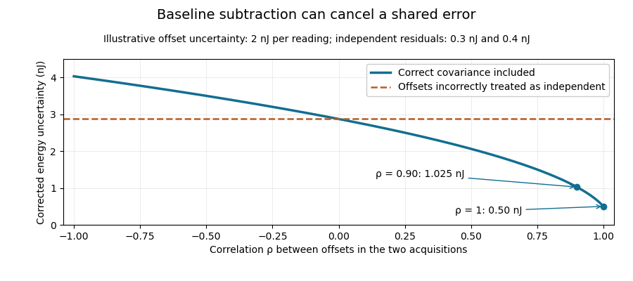
Shared baseline errors cancel according to their correlation
. Original numerical model with a 2 nJ offset uncertainty in each acquisition and independent residual uncertainties of 0.3 nJ and 0.4 nJ. The comparison curve incorrectly treats the shared offsets as independent. Details.A sampled implementation has the same structure. If a vector of readings has covariance matrix , and fixed integration weights give and , thenA constant offset cancels when the weights sum to the same gate duration: . This does not justify using pulse-contaminated readings as background. Matched blank sequences, collected with the actual timing, help characterize the needed noise correlations.
The historical NIST TC-24 apparatus used a thermocouple-based absorbing plate and averaged baseline measurements before and after laser injection to compensate background and thermal drift.[ref]
Calibration Service for Low-level Pulsed-Laser Radiometers at 1.06 µm: Pulse Energy and Peak Power by Rodney W. Leonhardt. §3.5, printed p. 8; §7.2, Leakage Effect
The offset model above is an independent illustration, not a reconstruction of that instrument's uncertainty budget.Reciprocal moments of an estimated variance determine whether a precision estimate such as has a finite expected value or variance. Small positive values of a sample variance become large values after inversion. An unbiased estimator of a variance therefore need not give an unbiased or even integrable estimate of its reciprocal.
For , let be independent normal random variables with common mean and variance . For the unbiased sample variance , put . Then has a chi-squared distribution. Its probability density function is for .[ref]
For any real , direct integration and the Gamma function giveThe convergence restriction is essential: near zero the integrand has exponent , so the integral diverges when . Substitution of a negative Gamma function argument into the displayed quotient does not define a nonexistent moment.
Rescaling gives the useful general resultIn particular, the mean reciprocal exists for , while its variance requires :For the mean is , the variance is and the coefficient of variation is . For the mean is finite but the variance is infinite. For even the mean diverges. Increasing the number of groups does not repair a nonexistent moment of each raw reciprocal estimate.
Inverse-variance weighting commonly normalizes these reciprocals. Those normalized weights lie between zero and one, so their moments can exist even when the raw reciprocal moments fail. This distinction matters in uncertainty in estimated inverse-variance weights: neither the moment calculation nor a plug-in precision formula alone establishes the accuracy of the final weighted estimator. The results here use the exact normal-sample law; a nonnormal sample requires a different analysis.
A vibrational frequency-state residence time is the duration a probe remains in a defined frequency environment before leaving it. It differs from the time over which the probe's frequency retains statistical memory, and from a vibrational relaxation lifetime describing excitation loss.
For a state with constant exit rate , let be the probability of no exit by time . The small-interval exit model givesThe residence-time density is , with mean and variance . The exponential distribution is memoryless: . These conclusions require a constant-rate model, rather than following from the name of a spectral state alone.
For a two-state continuous-time Markov chain with A-to-B rate and B-to-A rate , the mean residence times are and . The normalized two-state vibrational frequency memory instead decays as . Returning after an exit contributes to occupancy and correlation but not to survival without an exit.
An original symmetric example uses . Mean residence time is , while frequency-memory time is . Starting in A, the probability of being in A after iswhereas no-exit probability is . At these are about and .
This produces vibrational residence-time sampling bias if a same-state observation is treated as proof that no exit occurred. Using as an exit-rate estimate gives about , below the stipulated . Faster time sampling can resolve more excursions, but the estimator must still account for missed transitions and state-assignment uncertainty.
In two-dimensional infrared spectroscopy, the 2D IR waiting time separates initial frequency labeling from later response readout. Primary response theory relates such measurements to frequency memory under explicit approximations.[ref]
Frequency-frequency correlation functions and apodization in two-dimensional infrared vibrational echo spectroscopy: A new approach by Kyungwon Kwak and others. Introduction, pulse timing and frequency-frequency correlation function
A fitted memory decay is therefore not automatically a directly measured single-state residence time. Nonexponential survival can require additional states, time-dependent rates or a different physical model.The 3-torsion of an elliptic curve is the kernel of multiplication by three:with the field of points specified. If the characteristic is not three, the geometric group over an algebraic closure is and has nine points. The subgroup of points rational over the original field can be smaller.
For over , the point has order three. The tangent slope is , so the elliptic-curve doubling formulas give and hence . This displays a nonzero rational 3-torsion point rather than only asserting its possible existence.
In characteristic three, the geometric-point count need not be nine. The scheme-theoretic multiplication kernel still carries degree information not captured by counting its ordinary points. Thus the characteristic restriction is essential when identifying geometric 3-torsion with two cyclic groups.
The mixed fourth moment of thermal inputs measures how squared temperature and expansion-coefficient deviations occur together. For centered inputs and , defineIt has total input degree four. It is not the fourth moment of the product , which would involve . For a centered thermal product, the exact variance isConsequently individual input variances and their covariance do not in general determine the product variance.
For jointly normal centered inputs, write and using independent standard normal distributions. Expanding and using , and vanishing odd terms givesThis is a specific joint-Gaussian calculation, consistent with the Isserlis theorem; normal-looking marginals alone do not justify it.
An original bounded counterexample illustrates the extra information. Let equal with probabilities , and let an independent sign take equally. Put and . Both standardized marginals have mean zero and variance one, and , but . Replacing the second standardized input by an independent copy of preserves both marginals and zero covariance while changing to .
For an illustrative length correction , take , and . The two bounded models give standard deviations approximately14.14nm and10nm. Their factor-of-two variance difference comes entirely from joint occurrence, rather than changed marginal uncertainties.
NIST's thermal correction combines block length, expansion coefficient and temperature difference, providing the physical setting for this joint-input issue.[ref] Joint observations and the way coefficient or thermometer corrections are assigned must support the dependence model. Increasing the number of simulated draws cannot recover an unmeasured mixed moment. The GUM explicitly calls for higher-order treatment when a nonlinear response makes first-order propagation inadequate.[ref]
Asymptotic conservative Wald coverage under variance-ratio convergence requires the realized interval scale to be large enough in probability, together with a correctly centred limiting error law. The constant-ratio result in tail assumptions needed for conservative Wald coverage follows from Slutsky's theorem. A useful stronger formulation of the coverage conclusion needs no independence between centre and scale.
Let converge in distribution to a standard normal random variable, take , and let . If converges in probability to a constant , then for each , . ThereforeTaking the lower limit and then proves limiting coverage probability at least . In fact this lower-tail condition on suffices without convergence to one fixed constant. An expected-value inequality does not supply it; coverage failure under random variance-ratio limits can persist when the scale retains a substantial chance of being too small.
For an original comparison, choose . Under an exactly centred normal limit, a nominal 95 percent Wald confidence interval has limiting coverage . But if the standardized estimator instead converges to , the same scale givesA ten-percent increase in standard-error radius does not automatically cover an asymptotically material bias. These values use the normal cdf/ppf definitions.[ref]
SciPy 1.16.2 documentation. scipy.stats.norm, cdf and ppf
The result is pointwise in the assumed parameter/model sequence; it does not itself prove uniform coverage over a family of models or finite-sample accuracy. NIST's uncertainty guidance likewise conditions a confidence interpretation on the distributional justification, rather than on the multiplier alone.[ref]
The stress-optic coefficient measures the birefringence induced per unit principal-stress difference in the linear stress-optic law:Here is a difference of refractive indices, so has SI units . The wavelength matters: a coefficient determined with one illumination wavelength should not simply be reused with another. The signs of and also require a consistent ordering of the optical axes and stresses.[ref]
Experimental Strain Analysis by David Roylance. Printed p. 6, equation (5) and wavelength dependence
For a uniform specimen of thickness viewed along a principal optical direction, the measured phase retardation isA known uniaxial load supplies away from grips and other stress concentrations. Fitting the slope givesSubtracting the unloaded retardation removes a constant background, but a load-dependent background must be investigated rather than absorbed into the coefficient.
For an original illustrative measurement, let , and produce . ThenDoubling the stress difference doubles the retardation only within the same linear regime. This numerical value is illustrative, not a material specification.
An equivalent magnitude convention uses the photoelastic fringe value . One additional full retardation cycle corresponds to for the uniform model. A fringe magnitude alone does not determine the sign of or the separate principal stresses.
The Illinois primary apparatus description makes the measurement chain concrete: a leadscrew loads the specimen, a load cell measures force, monochromatic light passes through the specimen between polarizing elements, and a camera records fringes. Establishing connects those optical observations to a mechanical stress scale. Wavelength, thickness, unloaded birefringence and loading conditions belong with the reported coefficient.[ref]
Polariscope and Photoelasticity by the University of Illinois Mechanical Testing Instructional Laboratory. Specimen loading, monochromatic source, analyzer and camera
A Stein surface is a Stein manifold of complex dimension two, hence real dimension four. Its global holomorphic functions separate points and provide local coordinates, and the holomorphic hull of every compact subset is compact. The word “surface” here refers to complex dimension, rather than to a real two-dimensional surface.
The affine complex plane is a Stein surface, as is the smooth closed hypersurface in : its gradient never vanishes on the hypersurface. A compact connected positive-dimensional complex manifold cannot be Stein, because its holomorphic functions are constant. In real dimension four, the topology of Stein surfaces has especially rich links with handle decompositions and contact structures on three-dimensional boundaries.[ref]
Handlebody Construction of Stein Surfaces by Robert E. Gompf. Abstract and introduction, Stein surfaces and contact three-manifolds
The crossover from square-root to linear capacitive bridging bandwidth scaling occurs when excess error allowance becomes comparable with the resistive error floor itself. In square-root collapse of capacitive bridging bandwidth near the DC error floor, put , , , and . For positive , introduce the dimensionless ratio . The exact bandwidth can then be writtenThis single expression distinguishes the two regimes without exchanging small-parameter limits silently.
When and the tolerance is away from one, the factor is approximately : bandwidth scales as . When , that factor is approximately , while the denominator is close to one: bandwidth is approximately . The exactly zero-floor model has the corresponding small-tolerance linear behavior.
For an original dimensionless comparison, take . At , replacing by changes the numerator by only about . At , replacing it by changes the numerator by about ; here the total tolerance is , so the denominator differs little from one. The tolerance is small in both cases, but a different approximation is useful because its size relative to the floor differs.
In component terms, increasing moves the crossover by lowering ; changing only rescales the frequency axis through . A sweep of receiving electrical resistance and input capacitance can therefore separate a floor effect from a frequency-scale effect. The resistive/shunt-capacitive manufacturer model motivates the apparatus assumptions.[ref]
MT-040: Op Amp Input Impedance by Analog Devices. Printed pp. 1–2, input-path models and source-impedance dependence
The specification remains a full complex relative gain error, including phase shift, rather than only an amplitude or half-power threshold.This error combines two departures from an ideal sink prediction: resistance between the releasing surface and receiving liquid, and drug already present in that liquid. For the steady planar reservoir model in sink-boundary approximation error in drug release, let be the ideal flux, the mass-transfer Biot number for drug release and . Assume and , with concentrations expressed on compatible scales. ThenWriting the isolated resistance error as givesSimply adding and counts their overlap twice. For example, and give , rather than . This error uses the ideal flux as denominator; the overprediction relative to actual flux is .
A useful design calculation solves for how much bulk accumulation is permissible. For a requested tolerance ,The right side is nonnegative only if . Even zero initial bulk concentration cannot rescue too large an external resistance. At and , the permitted bulk fraction is about . For a maintained and a well-mixed receiving volume , this corresponds to about accumulated in the liquid, assuming no removal or other drug sources. This is an illustrative model calculation, not a general assay acceptance threshold.
Increasing receiving volume primarily limits ; changing flow or membrane transport can change . The FDA's adaptive-perfusion apparatus specifically replaces potentially rate-limiting passive membrane diffusion with pressure-driven tangential filtration.[ref]
Adaptive Perfusion: A Novel In Vitro Drug Release Testing Method for Complex Drug Products by the FDA. Technology Summary, conventional membrane transport versus pressure-driven separation
Comparing flow conditions and volumes can distinguish the two limitations. A finite reservoir, changing internal profile, partitioning or sampling requires its own mass balance before this steady expression can be interpreted as an error estimate.Burden voltage is the electric potential difference introduced between the terminals of an ammeter when an electric current flows through it. A shunt resistor makes a measurable signal by deliberately developing this drop, but the drop can also change the electric current being measured. In a real ammeter, leads, connections and a protection fuse can contribute as well as the shunt resistor.[ref]
Consider an ideal1volt source driving a100ohm resistor. Before inserting an ammeter, Ohm's law gives10milliamperes. If the inserted ammeter has10ohms of total series electrical resistance,The ammeter could report its own current perfectly and still measure a current9.09percent below the undisturbed value. This is a change in the measured electrical circuit, rather than a display-rounding error.
Reducing the shunt resistor's electrical resistance reduces burden voltage but also reduces the signal presented to an amplifier. A feedback ammeter instead uses a transimpedance amplifier to keep its input near a reference potential. National Instruments illustrates the distinction with a low-voltage leakage-current measurement, where the burden voltage consumes a substantial fraction of the applied test electric potential difference.[ref]
Minimizing Errors for Low-Current Measurements Using NI Hardware by National Instruments. Figures2–3 and associated leakage-current comparison
An experimental check uses several sensing resistors and records both the inferred electric current and the load's terminal electric potential difference. Dependence on the inserted electrical resistance reveals loading. Four-terminal sensing reduces errors from connection drops in the sensed signal; it does not remove the physical burden voltage across the shunt resistor.
Pinned article: Introduction to the OurBigBook Project
Welcome to the OurBigBook Project! Our goal is to create the perfect publishing platform for STEM subjects, and get university-level students to write the best free STEM tutorials ever.
Everyone is welcome to create an account and play with the site: ourbigbook.com/go/register. We belive that students themselves can write amazing tutorials, but teachers are welcome too. You can write about anything you want, it doesn't have to be STEM or even educational. Silly test content is very welcome and you won't be penalized in any way. Just keep it legal!
Intro to OurBigBook
. Source. We have two killer features:
- topics: topics group articles by different users with the same title, e.g. here is the topic for the "Fundamental Theorem of Calculus" ourbigbook.com/go/topic/fundamental-theorem-of-calculusArticles of different users are sorted by upvote within each article page. This feature is a bit like:
- a Wikipedia where each user can have their own version of each article
- a Q&A website like Stack Overflow, where multiple people can give their views on a given topic, and the best ones are sorted by upvote. Except you don't need to wait for someone to ask first, and any topic goes, no matter how narrow or broad
This feature makes it possible for readers to find better explanations of any topic created by other writers. And it allows writers to create an explanation in a place that readers might actually find it.
Figure 1. Screenshot of the "Derivative" topic page. View it live at: ourbigbook.com/go/topic/derivativeVideo 2. OurBigBook Web topics demo. Source. - local editing: you can store all your personal knowledge base content locally in a plaintext markup format that can be edited locally and published either:This way you can be sure that even if OurBigBook.com were to go down one day (which we have no plans to do as it is quite cheap to host!), your content will still be perfectly readable as a static site.
- to OurBigBook.com to get awesome multi-user features like topics and likes
- as HTML files to a static website, which you can host yourself for free on many external providers like GitHub Pages, and remain in full control

Figure 2. You can publish local OurBigBook lightweight markup files to either OurBigBook.com or as a static website.
Figure 3. Visual Studio Code extension installation.
Figure 5. . You can also edit articles on the Web editor without installing anything locally. Video 3. Edit locally and publish demo. Source. This shows editing OurBigBook Markup and publishing it using the Visual Studio Code extension. 
- Infinitely deep tables of contents:




All our software is open source and hosted at: github.com/ourbigbook/ourbigbook
Further documentation can be found at: docs.ourbigbook.com
Feel free to reach our to us for any help or suggestions: docs.ourbigbook.com/#contact