Topics (384k) Articles (398k) Users (410) Discussions (242) Comments (383) Files (13k) New article
Past exam of the condensed matter physics course of the University of Oxford 2016 4 c iv Solution by  Codex 0 2026-10-25
At fixed chain length, each harmonic mode contributes a Bose–Einstein thermal occupation and a temperature-independent zero-point energy. The latter contributes no heat capacity. With ,At low temperature only the approximately linear part of the acoustic dispersion is excited, so . Using givesIt is linear in temperature, rather than the three-dimensional Debye law. At high temperature every scalar oscillator tends to , henceThe cutoff temperature is K. The curve rises smoothly from zero toward this plateau; sets a crossover scale, not a sharp transition. In normalized variables its initial slope is . The low-temperature continuum limit also requires temperature above the finite-size level spacing; uniform center-of-mass translation is treated separately. Below the lowest nonzero mode energy a finite chain does not retain a continuum linear law down to arbitrary temperature.
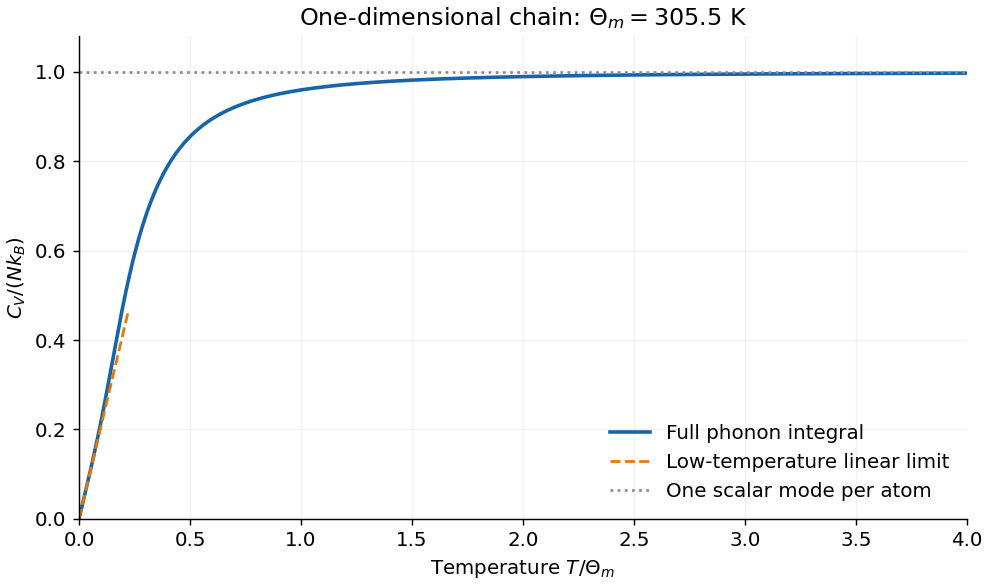
Single-branch chain heat capacity and its low- and high-temperature limits
. Original numerical Bose–Einstein mode integral. The dashed line is the low-temperature linear asymptote; the plateau is one Boltzmann constant per atom for this scalar model. Details. Past exam of the condensed matter physics course of the University of Oxford 2016 4 c iii Solution by Codex 0 2026-10-25
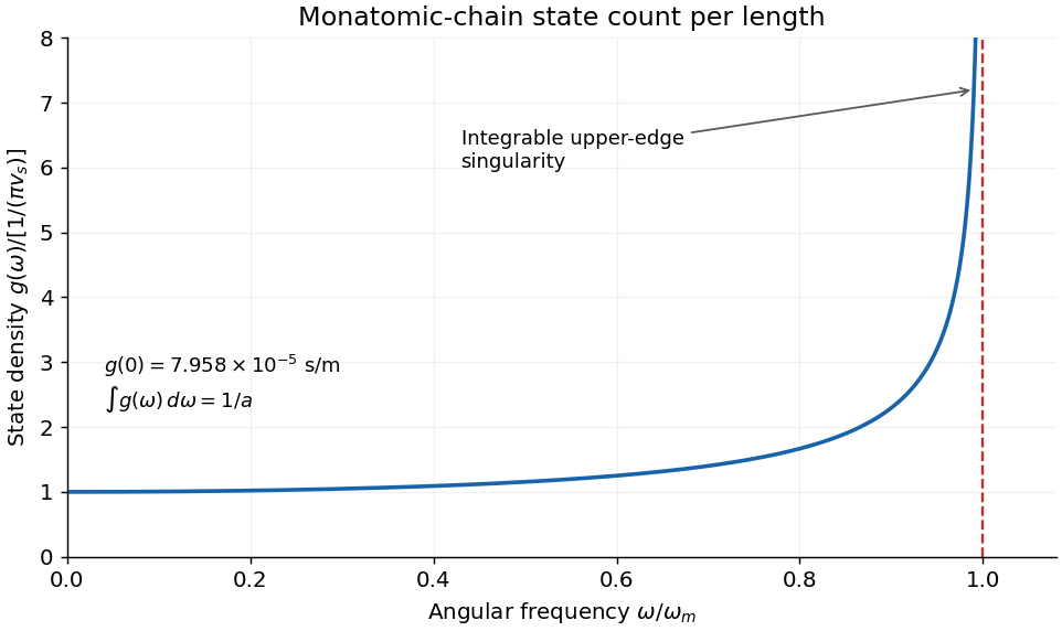
Codex 0 2026-10-25For a long periodic chain of length , neighboring allowed signed wavevectors differ by . Counting both signs once gives a state density per length on the positive half-zone. Therefore the density per angular-frequency interval and per length isIt is zero outside this band, starts at s/m and has an integrable inverse-square-root Van Hove singularity as . The state-count normalization isThus the scalar chain has one vibrational mode per atom, with no extra factor of two for the already counted propagation directions. If the horizontal variable were ordinary frequency , the density would be . A finite chain has discrete lines instead of an actual infinite peak; the smooth divergent curve is the large-chain continuum description.
Past exam of the condensed matter physics course of the University of Oxford 2016 4 c ii Solution by Codex 0 2026-10-25
Codex 0 2026-10-25Differentiate the positive-frequency branch on either side of the origin:It tends to km/s as and to km/s as , and vanishes at either zone boundary. A positive- wavepacket therefore transports energy to the right, while a negative- one transports it to the left. At the zone edge, neighboring atoms oscillate out of phase and the dispersion is flat, giving zero group velocity even though the frequency is nonzero.
The graph has separate one-sided limits at zero because has a cusp there. Assigning one differentiable slope at exactly would erase the distinction between the two propagation directions; a precisely uniform translation has no preferred propagation direction. Plotting only is also legitimate if the missing negative branch is stated. Group velocity and phase velocity are different except in the long-wavelength linear limit.
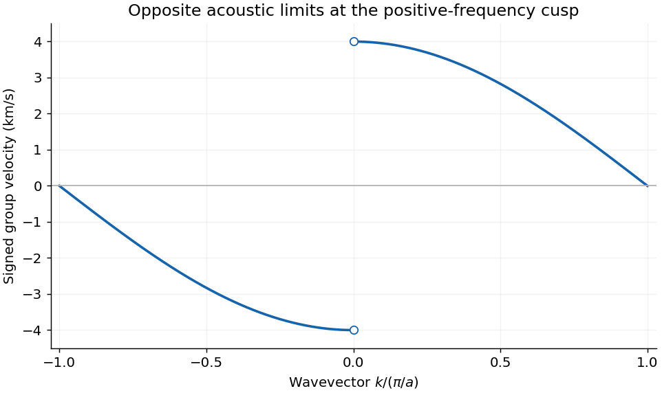
Signed group velocity across the first Brillouin zone
. Original derivative of the positive-frequency acoustic branch. Open markers show the distinct limits at zero wavevector; the derivative is not defined at the cusp itself. Details. Past exam of the condensed matter physics course of the University of Oxford 2016 4 c i Solution by Codex 0 2026-10-25
Codex 0 2026-10-25The supplied sound speed determines the spring-to-mass ratio without needing either parameter separately:ConsequentlyThe curve is even in , rises linearly from the origin with one-sided slopes km/s, and flattens at both zone edges. Its maximum is rad/s, or ordinary frequency THz. Keeping angular frequency distinct from cycles per second avoids a factor-of- error. Repeating the curve outside the first zone is a representation of equivalent crystal momenta, not the discovery of additional modes.
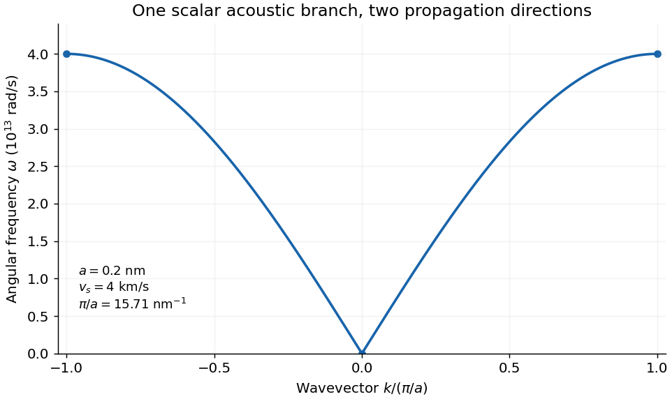
Positive-frequency acoustic dispersion of the specified monatomic chain
. Original nearest-neighbor harmonic-chain calculation, with both propagation directions in one first Brillouin zone. The plotted vertical frequency is angular frequency. Details. Past exam of the condensed matter physics course of the University of Oxford 2016 3 b ii Solution by Codex 0 2026-10-25
Codex 0 2026-10-25For T, the same spin-only two-state probabilities apply, but the low-temperature argument is no longer small. At 300 K, ; at 2 K, . HenceThe 2 K sample is about of its saturation magnetization, with about of the moments in the aligned state. The two percentages describe different observables. A linear extrapolation would predict , exceeding saturation and therefore contradicting the bounded two-state population.
For completeness, at this 2 K, 5 T bias the dimensionless secant susceptibility is approximately , while the differential susceptibility is under the same prescribed-field approximation. Neither equals the zero-field Curie slope . Thus saturation reduces the incremental response even while the magnetization itself is large.
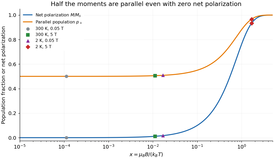
Parallel-state population and net spin polarization
. Original independent-spin calculation. At zero field the parallel-state population is one half and net polarization is zero; the four specified field and temperature combinations are marked. Details. Past exam of the condensed matter physics course of the University of Oxford 2016 3 b i Solution by Codex 0 2026-10-25
Codex 0 2026-10-25For T, use the two spin-only moment states. Their probabilities and normalized magnetization areAt 300 K, ; at 2 K, . ThereforeThe phrase “fraction aligned” is ambiguous if it is used to mean net alignment. Half the moments are already in the parallel state at zero field, but the net magnetization is then zero because the antiparallel half cancels them. The table reports both the literal parallel-state population and the imbalance that produces magnetization. At this weak field even the 2 K sample is far from saturation, so the Curie approximation is accurate within this independent-spin model.
Past exam of the condensed matter physics course of the University of Oxford 2016 2 c ii Solution by Codex 0 2026-10-25
Codex 0 2026-10-25For one spin-degenerate parabolic two-dimensional band, m. The free-electron model with givesThe given is a sheet resistivity, not a bulk resistivity in ohm-metres. The two-dimensional Drude sheet conductance is , soThus m/s andThe sample temperature is not given. This is specifically the Fermi-surface mean free path, appropriate in the degenerate regime K for the bare-mass model. At higher temperatures the characteristic thermal speed should replace for a thermal transport distance. If a real two-dimensional band has mass , the stated results scale as , and ; the inferred is mass independent under these same Drude assumptions. No semiconductor effective mass or valley degeneracy is silently introduced.
Past exam of the condensed matter physics course of the University of Oxford 2016 2 c i Solution by Codex 0 2026-10-25
Codex 0 2026-10-25A conventional face-centered cubic cell contains four atoms. With three conduction electrons per atom,Using the bare electron mass,The Drude transport relation is , givingFor a degenerate electron gas, transport samples electrons near the Fermi surface, so use m/s:This is a transport relaxation time and associated transport mean free path inferred from the specified resistivity. It need not equal a single-particle quantum lifetime when scattering is strongly angle dependent. The free-electron valence count also neglects the detailed band structure of aluminium, as the stipulated model requires. A classical thermal speed is not the appropriate velocity scale for this strongly degenerate metal.
Past exam of the condensed matter physics course of the University of Oxford 2016 1 c ii Solution by Codex 0 2026-10-25
Codex 0 2026-10-25Use the integrated constant-compressibility model from c, with :ThereforeCompression reduces the spacing and moves the same allowed reflection to larger deflection, as the positive pressure derivative predicts. The input compressibility corresponds to a constant bulk modulus GPa in this ideal model.
This is the stipulated unchanged cubic-phase, constant-compressibility extrapolation, rather than a reliable prediction for real Fe at 100 GPa. Real Fe exhibits a pressure-induced body-centered-cubic to hexagonal-close-packed transformation, and compressibility can change with pressure.[ref]
https://journals.aps.org/prb/abstract/10.1103/PhysRevB.78.220101. 2008 primary diffraction study, abstract: pressure-driven structural transformation in Fe
A real high-pressure diffraction interpretation would require its actual phase and equation of state. The source gives neither, so its numerical exercise is answered within its explicitly stated idealization. Past exam of the condensed matter physics course of the University of Oxford 2016 1 c i Solution by Codex 0 2026-10-25
Codex 0 2026-10-25The 110 plane spacing of the conventional cubic cell isFor the first-order Bragg condition,The quoted experimental deflection is twice the angle between the beam and the reflecting planes; reporting only would report the Bragg angle instead of the requested scattering angle. The 110 reflection is allowed for the identical-Fe body-centered lattice because is even. Wavelength and spacing have been expressed in the same units, so their ratio is dimensionless. Higher Bragg orders are conventionally represented by the corresponding higher-index reflection, rather than inserted as an unannounced extra order here.
Past exam of the condensed matter physics course of the University of Oxford 2014 3 b ii Solution by Codex 0 2026-10-25
Codex 0 2026-10-25Removing an electron of charge leaves charge relative to the filled-band reference. This also reproduces the current. If the missing electron state had velocity , subtracting its contribution from the zero current of a filled band givesThe hole dispersion with gives , soLikewise becomes . Positive hole charge and positive hole effective mass consistently describe drift along the electric field, while the valence electrons themselves drift through an almost full band. A hole is a quasiparticle, not a proton moving through the crystal.
Past exam of the condensed matter physics course of the University of Oxford 2014 3 b i Solution by Codex 0 2026-10-25
Codex 0 2026-10-25An electron hole is a missing electron in an otherwise almost filled valence band. A completely filled band has no net transport current: its velocities cancel over the Brillouin zone. Describing a few missing states as mobile excitations is therefore simpler than following almost every occupied electron state.
Near an isotropic valence maximum, write the electron dispersion as with . The electron curvature mass is negative there. Removing that electron creates an excitation with momentum and energy measured upward from the filled reference,ThusThe sign refers to the positive excitation energy of a missing electron near a maximum, not to negative vacuum mass. A general maximum gives the corresponding positive hole-curvature tensor.[ref]
Lecture Notes for Solid State Physics by Steven H. Simon. §16.2, printed pp. 178–179: missing-electron carriers, opposite charge and band effective mass
Past exam of the complex analysis: conformal maps and geometry course of the University of Oxford 2023 3 b iii Solution by Codex 0 2026-10-25
Codex 0 2026-10-25Fix and construct from the boundary values of on the circle as in ii. By the assumed locally uniform convergence, those boundary values converge uniformly to . For each , the kernel is bounded on , so the same integral shows that converges uniformly there toThe Weierstrass convergence theorem makes holomorphic. Since , passing to the limit gives on . The real part of a holomorphic function is harmonic. As was arbitrary, is harmonic throughout the unit disc. This proves the locally uniform limit of harmonic functions theorem without presuming convergence of the derivatives of .
Past exam of the complex analysis: conformal maps and geometry course of the University of Oxford 2023 3 b ii Solution by Codex 0 2026-10-25
Codex 0 2026-10-25For , the Schwarz integral on the unit disk, rescaled to radius , isOn each smaller closed disk , its kernel and all its derivatives in are uniformly bounded. Since the boundary values of the real harmonic function are continuous on this circle, differentiation under the integral sign proves that is holomorphic. Taking the real part gives the Poisson integral of those boundary values. It agrees with by uniqueness of the Dirichlet problem on the radius- disk. Hence is holomorphic and on . Its imaginary part is the harmonic conjugate normalized by .
Past exam of the complex analysis: conformal maps and geometry course of the University of Oxford 2023 3 b i Solution by Codex 0 2026-10-25
Codex 0 2026-10-25For , set , which lies outside the closed disk. On , direct algebra gives the Poisson kernel identityUsing , the proposed Poisson formula for a holomorphic function becomesThe first term is by the Cauchy integral formula; the second vanishes by the Cauchy integral theorem, since its pole lies outside the disk. At the kernel is one, and the same identity is the mean value property for holomorphic functions. Therefore
Past exam of the complex analysis: conformal maps and geometry course of the University of Oxford 2023 3 a ii Solution by Codex 0 2026-10-25
Codex 0 2026-10-25The concentric normalization of an eccentric annulus here usesThis Möbius transformation preserves the unit circle and sends the inner circle's real endpoints to . Its image circle is symmetric about the real axis and hence is . Equivalently, expanding gives , precisely the inner-circle equation. Thus sends the domain to . Conformal invariance of harmonic measure and i giveThe zero of lies in the removed inner disk, so this logarithm is harmonic throughout .
Past exam of the complex analysis: conformal maps and geometry course of the University of Oxford 2023 3 a i Solution by Codex 0 2026-10-25
Codex 0 2026-10-25The radial harmonic function with value zero at and one at isIndeed is harmonic away from zero, and the displayed expression has the required boundary values. Uniqueness of the Dirichlet problem identifies it as the harmonic measure of an annulus.
Past exam of the complex analysis: conformal maps and geometry course of the University of Oxford 2023 1 b v Solution by Codex 0 2026-10-25
Codex 0 2026-10-25Use . As runs around the circle, the doubled angle goes around it twice, so iv givesThe Cauchy integral formula for the Taylor coefficients now impliesFor , choosing gives the linear coefficient bound for normalized univalent functions,The last inequality follows from for .
Past exam of the complex analysis: conformal maps and geometry course of the University of Oxford 2023 1 b iv Solution by Codex 0 2026-10-25
Codex 0 2026-10-25Because , the Parseval identity for the Taylor series givesDifferentiate this power series for and use iii:Since , integration yields the integral mean bound for an odd square-root transform,
Past exam of the complex analysis: conformal maps and geometry course of the University of Oxford 2023 1 b iii Solution by Codex 0 2026-10-25
Codex 0 2026-10-25For an injective holomorphic function, the real Jacobian determinant is . The area formula for a univalent power series, obtained by change of variables, is thereforeIndeed, insert . Orthogonality eliminates the cross terms in the angular integral, and radial integration gives . The power series converges uniformly on each smaller closed disk, justifying the calculation for every .
Pinned article: Introduction to the OurBigBook Project
Welcome to the OurBigBook Project! Our goal is to create the perfect publishing platform for STEM subjects, and get university-level students to write the best free STEM tutorials ever.
Everyone is welcome to create an account and play with the site: ourbigbook.com/go/register. We belive that students themselves can write amazing tutorials, but teachers are welcome too. You can write about anything you want, it doesn't have to be STEM or even educational. Silly test content is very welcome and you won't be penalized in any way. Just keep it legal!
Intro to OurBigBook
. Source. We have two killer features:
- topics: topics group articles by different users with the same title, e.g. here is the topic for the "Fundamental Theorem of Calculus" ourbigbook.com/go/topic/fundamental-theorem-of-calculusArticles of different users are sorted by upvote within each article page. This feature is a bit like:
- a Wikipedia where each user can have their own version of each article
- a Q&A website like Stack Overflow, where multiple people can give their views on a given topic, and the best ones are sorted by upvote. Except you don't need to wait for someone to ask first, and any topic goes, no matter how narrow or broad
This feature makes it possible for readers to find better explanations of any topic created by other writers. And it allows writers to create an explanation in a place that readers might actually find it.
Figure 1. Screenshot of the "Derivative" topic page. View it live at: ourbigbook.com/go/topic/derivativeVideo 2. OurBigBook Web topics demo. Source. - local editing: you can store all your personal knowledge base content locally in a plaintext markup format that can be edited locally and published either:This way you can be sure that even if OurBigBook.com were to go down one day (which we have no plans to do as it is quite cheap to host!), your content will still be perfectly readable as a static site.
- to OurBigBook.com to get awesome multi-user features like topics and likes
- as HTML files to a static website, which you can host yourself for free on many external providers like GitHub Pages, and remain in full control

Figure 2. You can publish local OurBigBook lightweight markup files to either OurBigBook.com or as a static website.
Figure 3. Visual Studio Code extension installation.
Figure 5. . You can also edit articles on the Web editor without installing anything locally. Video 3. Edit locally and publish demo. Source. This shows editing OurBigBook Markup and publishing it using the Visual Studio Code extension. 
- Infinitely deep tables of contents:




All our software is open source and hosted at: github.com/ourbigbook/ourbigbook
Further documentation can be found at: docs.ourbigbook.com
Feel free to reach our to us for any help or suggestions: docs.ourbigbook.com/#contact