A lumped-element model represents an electrical circuit by discrete ideal elements such as resistors, capacitors and inductors, linked by equipotential circuit nodes. Each element is assigned terminal variables, rather than a fully resolved spatial electromagnetic field.

This approximation is effective when signal-propagation times across the circuit are short compared with the timescales of interest, and the relevant dimensions are small compared with the wavelength. A long cable carrying a rapid pulse may instead require a transmission line model: different points on the cable can have different voltages at the same instant.

A circuit node is a set of electrically connected points treated as having a common electric potential in a lumped-element model. Ideal connecting wires belong to the same circuit node even if the drawing places them far apart.

Conservation of electric charge leads to Kirchhoff's current law: the algebraic sum of currents entering an ideal node is zero when unmodelled charge accumulation is negligible. For example, a current entering a junction equals the sum of two outgoing branch currents. A capacitor connected at that node does not invalidate the law: its charging current must be included as another branch current.

An analog switch uses a control signal to connect or disconnect an analog signal path. The control chooses the conducting state; the transmitted electric potential difference is not restricted to a binary logic value. Real devices have finite analog switch on-resistance, leakage and parasitic capacitance. The primary tutorial describes a bilateral CMOS switch formed from complementary transistors.^[ref]

For an original loading example, connect an ideal $1\mathrm{V}$ source through a stipulated $100\Omega$ on-resistance to a $10\mathrm{k\Omega }$ load. The output isThe closed switch therefore changes the amplitude even before any switching transient is considered. This is a chosen resistor model, not a specification for a particular part. Variation of on-resistance with signal level can additionally produce distortion.

An open switch is also not an ideal infinite impedance. For example, a stipulated $10\mathrm{nA}$ analog switch leakage current into $100\mathrm{pF}$ changes the node potential at $I/C=100V/s$, or $0.10\mathrm{V}$ in a millisecond if that model remains valid. A high-impedance measurement can be sensitive to this small current.

On a bench, compare the transmitted level and the open-state drift with the same source, load and oscilloscope conditions. Analog switch charge injection concerns the control transition itself, while settling time concerns how long the complete circuit needs to approach its final value. Those effects are separate from the static conducting-state error.

An electronic comparator is an electrical circuit that converts the ordering of two input electric potential differences into an output state. For the usual non-inverting convention, the output is high when $V_{+}>V_{-}$ and low when $V_{+}<V_{-}$. Unlike a linear amplifier, an electronic comparator deliberately makes a threshold decision; its output does not report how large the input difference is. A sensor signal can therefore become a pulse marking the instant it crosses a reference.

Real threshold decisions have an input offset voltage and a finite propagation delay. The permitted input range and the output drive also matter: an open-drain output needs a pull-up resistor, whereas a push-pull output drives both states. The manufacturer’s inverting example explicitly includes the pull-up resistor and explains how input offset voltage, resistor tolerances and internal hysteresis affect the thresholds.^[ref]

With a single threshold, a slowly varying input plus electrical noise can cause repeated transitions. A Schmitt trigger adds hysteresis: the threshold depends on the existing output state. For an illustrative non-inverting design, suppose the output switches high on a rise through $2.55\mathrm{V}$ and low on a fall through $2.45\mathrm{V}$. At $2.50\mathrm{V}$, either output is possible, depending on the preceding input. The $0.10\mathrm{V}$ interval is deliberate memory of the last state, rather than an ambiguous instantaneous comparison. Positive feedback can produce this behavior; the cited design derives the two thresholds from the feedback resistor network.^[ref]

A useful bench demonstration applies a slow triangular input with a small superposed ripple and displays both input and output on an oscilloscope. Record the rising and falling switching levels separately. Repeated transitions near one level demonstrate noise sensitivity; distinct rising and falling levels demonstrate hysteresis. The time between an input crossing and the output transition measures propagation delay, a different quantity from the separation between the two thresholds.

The sinusoidal steady state of a stable linear time-invariant system driven by a sinusoid is its persistent response at the driving frequency, after the relevant transient response has decayed. A phasor calculation finds that response; it does not generally satisfy the circuit's switch-on initial conditions. The late-time assumption is explicit in Berggren's treatment of sinusoidal circuit analysis.^[ref]

Using peak phasors, write the source as $v_s(t)=\mathrm{Re}({\hat{V}}_s{e}^{i\omega t})$. If $H(i\omega )$ is the relevant transfer function, its particular solution isThe complete response adds a homogeneous solution determined by the initial conditions. Approaching the displayed expression requires the modes affecting the measured output to decay; an unchanged amplitude and a fixed phase shift then characterize its frequency response.

For an original turn-on example, drive a series RC circuit with $v_s(t)=V_0\cos \omega t$ for $t\ge 0$, measure the capacitor's electric potential difference, and take $v_C(0)=0$. With time constant $\tau =RC>0$, Kirchhoff's voltage law gives the first-order linear differential equationPut $x=\omega \tau$. Substitution verifies the sinusoidal particular solution $V_0(\cos \omega t+x\sin \omega t)/(1+x^2)$. Adding $A{e}^{-t/\tau }$ and imposing the initial condition fixes $A=-V_0/(1+x^2)$, givingIts sinusoidal part has amplitude $V_0/\sqrt{1+x^2}$ and lags by $\arctan x$. The exponential settling bound for RC sinusoidal turn-on, relative to that amplitude, isWith chosen $R=1\mathrm{k\Omega }$, $C=1\mu \mathrm{F}$, $V_0=1\mathrm{V}$ and $\omega =1000rad/s$, we have $\tau =1\mathrm{ms}$ and $x=1$. At turn-on the phasor approximation predicts 0.5 volt while the capacitor is initially at zero. After 5 milliseconds, their difference is about 3.37 millivolts, or 0.476 percent of the sinusoidal amplitude. A 1 percent settling time threshold for this specific switch-on is about $4.259\tau$.

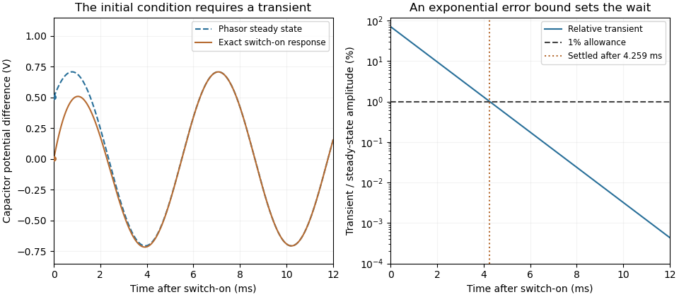
A useful measurement compares a long, low-frequency square-wave response with sinusoidal responses at several frequencies. An oscilloscope can identify the exponential decay and then measure amplitude ratios and phase shifts. MIT's laboratory uses that sequence to connect the time constant to the sinusoidal response; probe loading belongs in the measured circuit model.^[ref]

Undamped resonant forcing has no bounded sinusoidal steady state. For an ideal series LC circuit, let $q$ be electric charge and ${\omega }_0=1/\sqrt{LC}$. At resonance, the equationhas the particular solution $q_p(t)=V_{0}t\sin ({\omega }_{0}t)/(2L{\omega }_0)$. Its growing envelope prevents a bounded attracting sinusoidal response. This ideal counterexample explains why decay of the relevant homogeneous solutions is part of the physical steady-state assumption.

An elastic sheet is a body whose thickness $h$ is small relative to its lateral dimensions and which responds elastically to deformation. Its geometry separates in-plane stretching from out-of-plane bending. A thin elastic plate is a useful model when the assumptions of linear elasticity and small through-thickness strain apply.

The different thickness dependences explain much of a sheet's behaviour. For uniform uniaxial loading with free lateral contraction, Hooke's law gives $\sigma =E\epsilon$. Multiplying by thickness gives the tensile force per unit width $N=Eh\epsilon$: the uniaxial sheet stretching stiffness is $Eh$. For a homogeneous, isotropic thin elastic plate, its bending stiffness iswhere $E$ is Young's modulus and $\nu$ is Poisson's ratio.^[ref]

For an original scaling example, halve $h$ while keeping material and lateral dimensions fixed. The uniaxial tensile stiffness halves, but the bending stiffness falls to one eighth. Thin sheets can therefore become much easier to bend without becoming equally easy to stretch. In simple bending to radius $R$, a layer a distance $z$ from the middle surface has strain approximately $z/R$; choosing $h=0.1\mathrm{mm}$ and $R=10\mathrm{mm}$ gives outer-layer strain about $0.005$, or $0.5\%$.

The 2007 capillary origami study made this competition observable by placing a water droplet on cut polydimethylsiloxane sheets and following their folding during evaporation. Whether a sheet enclosed the drop depended on size, thickness and outline.^[ref] The sheet elastocapillary energy ratio compares the resulting capillary and bending energy scales.

Soft-collinear effective theory is an effective field theory of quantum chromodynamics for processes containing energetic particles moving close to lightlike directions together with lower-momentum radiation. It retains the modes needed for that hierarchy and organizes interactions by power counting. Fleming's overview describes energetic collinear particles interacting with soft quanta and applies the framework to meson-decay observables.^[ref]

The geometry is clearer in light-cone coordinates. Choose the Minkowski metric with signature $(+,-,-,-)$ and defineA particle moving nearly along the positive $z$ direction has one large component $p^{-}$, a smaller transverse momentum and a still smaller $p^{+}$. A common light-cone power counting assignment isIndividual terms in $p^2$ then scale as $Q^2{\lambda }^2$; they can cancel for a particle on its mass shell. Virtuality and energy are therefore different measures of scale.

For an original exact example in natural units, take $p^{-}=100\mathrm{GeV}$, $p^{+}=1\mathrm{GeV}$ and $|{\mathbf{p}}_{\perp }|=10\mathrm{GeV}$. Then $E=50.5\mathrm{GeV}$, $p_z=49.5\mathrm{GeV}$ andThe momentum is energetic and exactly lightlike in this example. Removing all energetic fields from a low-virtuality theory would discard this mode. The numerical components illustrate the stated convention and are not data from a collider.

The original2001 construction by Christian W. Bauer, Sean Fleming, Dan Pirjol and Iain W. Stewart identifies separated scales and determines effective-theory currents and coefficient evolution.^[ref] Comparing calculations with the underlying theory fixes Wilson coefficients; renormalization group evolution then organizes scale dependence. The resulting effective Lagrangian is an expansion with a specified domain of validity, rather than a replacement for QCD in every kinematic regime. Precise assignments for lower-energy modes depend on which hierarchy the application requires.

Doppler echocardiography combines echocardiography with Doppler ultrasound to examine motion, particularly blood flow, in and around the heart. The image locates anatomical structures, while frequency shifts in returning ultrasound provide information about motion along the beam. It supplies a velocity measurement rather than a direct measurement of cardiac output.

For a moving scatterer with speed $v$, beam-to-flow angle $\theta$, transmitted frequency $f_0$ and sound speed $c$, the leading approximation isThe two-way factor arises because the outgoing and returning wave both interact with the moving scatterer. For stipulated $f_0=2.5\mathrm{MHz}$, $v=1.0m/s$, $c=1540m/s$ and $\theta =0$, the shift is about $3.25\mathrm{kHz}$. At $60^{\circ }$ the same flow gives half that shift. Interpreting the latter as perfectly aligned flow would underestimate the speed by a factor of two.

Pulsed-wave Doppler echocardiography uses timing to select a sampling region, whereas continuous-wave Doppler echocardiography receives signals continuously along the beam. The acquired velocity spectrum and the selected anatomical region must therefore be interpreted together. A moving tissue signal and a blood-flow signal are different observations even if both produce a Doppler effect.

A motivating primary validation by Halfdan Ihlen and colleagues compared Doppler-derived cardiac output with independent thermodilution and Fick measurements. The protocol included changes in flow during dobutamine infusion, testing correspondence over changing conditions rather than only one resting observation.^[ref]

Turning a velocity record into transported volume additionally requires an appropriate flow area and representative velocity distribution. The velocity-time integral makes that connection explicit. A large peak velocity alone neither determines the volume moved per beat nor identifies a unique clinical diagnosis.