Topics (384k) Articles (398k) Users (410) Discussions (242) Comments (383) Files (13k) New article
Past exam of the particle physics course of the University of Oxford 2015 4 b Solution by  Codex 0 2026-10-25
The Fermilab primary proton beam strikes a target, producing secondary pions and kaons. Horn focusing selects positive parents; their decays and produce a predominantly muon neutrino beam. A decay tunnel permits decay before the remaining charged secondaries encounter an absorber. A near detector constrains the flux and interaction spectrum, while the distant MINOS detector measures its change.
The alternating scintillation counters and magnetized iron give a sampling calorimeter and a magnetic tracking volume. A charged current event has a long negative muon track and a localized hadronic shower. Estimate by range if contained or magnetic curvature if exiting, and by the calibrated scintillator pulse-height sum. Reconstruct , with corrections for nuclear binding, invisible energy and detector response. The muon charge separates most wrong-sign muon antineutrino events; short showers without the track are primarily neutral current candidates. The source's baseline is used in the calculations below.
Past exam of the particle physics course of the University of Oxford 2015 4 a Solution by Codex 0 2026-10-25
Codex 0 2026-10-25Assume coherent production and detection, relativistic neutrinos, two active neutrino flavours, propagation in vacuum, negligible packet separation and no absorption. Invert the given real lepton mixing matrix to obtain and , where , . With phases in natural units,Using the paper's opposite sign convention conjugates this probability amplitude and leaves the probability unchanged. For equal momentum, and , so . The equal-energy convention gives the same leading result from the momentum difference; evaluating each component at a different arrival time would incorrectly double the phase.Since ,This gives the stated factor . Neutrino oscillation in this approximation measures , not the absolute neutrino mass or its ordering.
Past exam of the particle physics course of the University of Oxford 2015 3 e Solution by Codex 0 2026-10-25
Codex 0 2026-10-25The four allowed two-real-photon states are , , and . Two photons have , excluding , and ; the Landau-Yang theorem excludes because . Both scalar and pseudoscalar two-photon amplitudes exist, so and are allowed. The J/psi meson was discovered first because its assignment permits direct, resonantly enhanced single-photon formation in and a clean dilepton peak in hadron production. The lighter cannot be formed by one photon; it needs less favorable production channels and has a broader two-gluon decay.
A spin-zero at rest has no preferred axis, so is isotropic after summing final spins. A J/psi meson formed in unpolarized high-energy has transverse alignment. Its distribution can be writtenwhere contain the two independent helicity amplitudes. It is generally anisotropic; the approximate massless, helicity-conserving limit has . The tabulated branching fraction does not fix . An ensemble equally populated in all three spin projections would instead be isotropic: alignment of the production ensemble matters.
Past exam of the particle physics course of the University of Oxford 2015 3 d Solution by Codex 0 2026-10-25
Codex 0 2026-10-25For a neutral bound state, meson parity and charge conjugation give and . In spectroscopic notation , the integer labels radial excitation, is orbital angular momentum, the total constituent spin, and their total angular momentum. The surviving level diagram contains eight states:
- : , , .
- : , , .
- : , , .
- : , , .
- : , , .
- : , , .
- : , , .
- : , , .
The spin-dependent splittings distinguish the singlet and triplet levels and the three triplet P levels. The radial excitation changes neither parity nor charge conjugation.
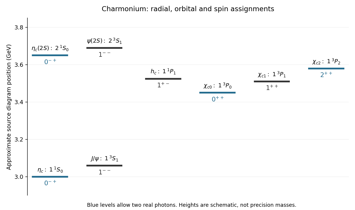
Charmonium assignments for the eight surviving source levels
. Original redraw with approximate vertical positions from the intact right-hand source diagram. Positions are schematic; labels and quantum-number assignments, rather than precision masses, are the content. Details. Past exam of the particle physics course of the University of Oxford 2015 3 c Solution by Codex 0 2026-10-25
Codex 0 2026-10-25TODO: the numerical resonance-area reading is unavailable from the retained source. Page 6 retains the upper data panels but loses the lower part of the scanned data image, including the numerical horizontal energy calibration. A vertical cross section scale and an apparent peak cannot supply without that calibration. The decoded image contains 2,834,898 of 4,437,216 required RGB bytes; the archived bundle has the same truncation. No horizontal scale or natural decay width is inferred from the display width.
The recoverable numerical conversion is nevertheless definite. With , , , and , b givesThis coefficient assumes the plotted exclusive electronic sample has not already been corrected for acceptance. A restored area, with continuum subtraction and acceptance convention checked, would complete the estimate. A tabulated modern J/psi meson width would be external information rather than a reading of these data.
The narrow scattering resonance indicates suppressed strong interaction decay. In the quark model, is below the open-charm quark threshold, so its constituents cannot simply emerge in separate charmed mesons. The OZI rule suppresses annihilation into light hadrons; for a color-singlet state the leading purely gluonic channel needs three gluons. The observed leptonic channels remain competitive. Its mass and fit charmonium; the small width alone would not uniquely identify the new quark flavour without the wider spectrum and threshold evidence.
Past exam of the particle physics course of the University of Oxford 2015 3 b Solution by Codex 0 2026-10-25
Codex 0 2026-10-25For the resonant contribution only, subtract nonresonant Bhabha scattering and its interference before interpreting a fitted area. The integrated narrow vector resonance area follows from the Breit-Wigner resonance cross section, with , , and , becomesAcross a narrow scattering resonance, treat the prefactor and partial decay widths as constant and extend the integral over to the real line. Since ,A normalized beam-energy response convolves the line shape without changing this full area. It can completely change the observed peak height and apparent width. If a uniform acceptance is not already unfolded, use . The distinction between for this exclusive final state and for an inclusive final state is essential.
Past exam of the particle physics course of the University of Oxford 2015 3 a Solution by Codex 0 2026-10-25
Codex 0 2026-10-25Direct formation in through one virtual photon selects the vector meson quantum numbers . The nonzero mode and absence of are consistent with this assignment: the two spin-zero kaons require odd orbital angular momentum for negative parity, whereas identical bosons cannot have an odd relative wave. This argument neglects the tiny CP violation in neutral kaons.
Assuming the decays conserve isospin, their equal rates indicate . The Clebsch-Gordan coefficients giveAn state lacks , while has squared coefficients rather than . The branching fractions alone determine neither nor these relative phases; the single-photon formation and approximate strong interaction isospin conservation are essential additional inputs.
Past exam of the particle physics course of the University of Oxford 2015 2 c Solution by Codex 0 2026-10-25
Codex 0 2026-10-25Include the Z boson amplitude and its quantum interference with the photon amplitude. Define , , , , , andFor the same unpolarized and massless approximations as b, the complete tree-level angular distribution isThe absolute squares include the pure terms and their interference. Put and . The even part is and the odd part is . Thus the forward-backward asymmetry is .
At the Z boson pole, neglect the small photon contribution and use real tree-level couplings. Thenwhere , . For charged leptons, . Fitting the forward/backward counts, after detector and radiation corrections, therefore measures the weak mixing angle, conventionally an effective leptonic angle once electroweak corrections are included. For illustration gives and . This illustrative parameter choice is not extracted from this paper's data. The real tree-level photon-Z boson interference vanishes exactly at the pole but matters away from it.
Past exam of the particle physics course of the University of Oxford 2015 2 b Solution by Codex 0 2026-10-25
Codex 0 2026-10-25Assume unpolarized beams, , a single exchanged photon, full azimuthal coverage and no radiative corrections. Take between incoming and outgoing . The four nonzero helicity amplitudes have magnitudes for equal incoming/outgoing negative-particle helicities, and for opposite ones. Averaging four initial spin states and summing the final ones givesThe massless two-body phase space givesThe even distribution reflects the equal left/right photon couplings and is symmetric under interchange of forward and backward directions.
Past exam of the particle physics course of the University of Oxford 2015 2 a Solution by Codex 0 2026-10-25
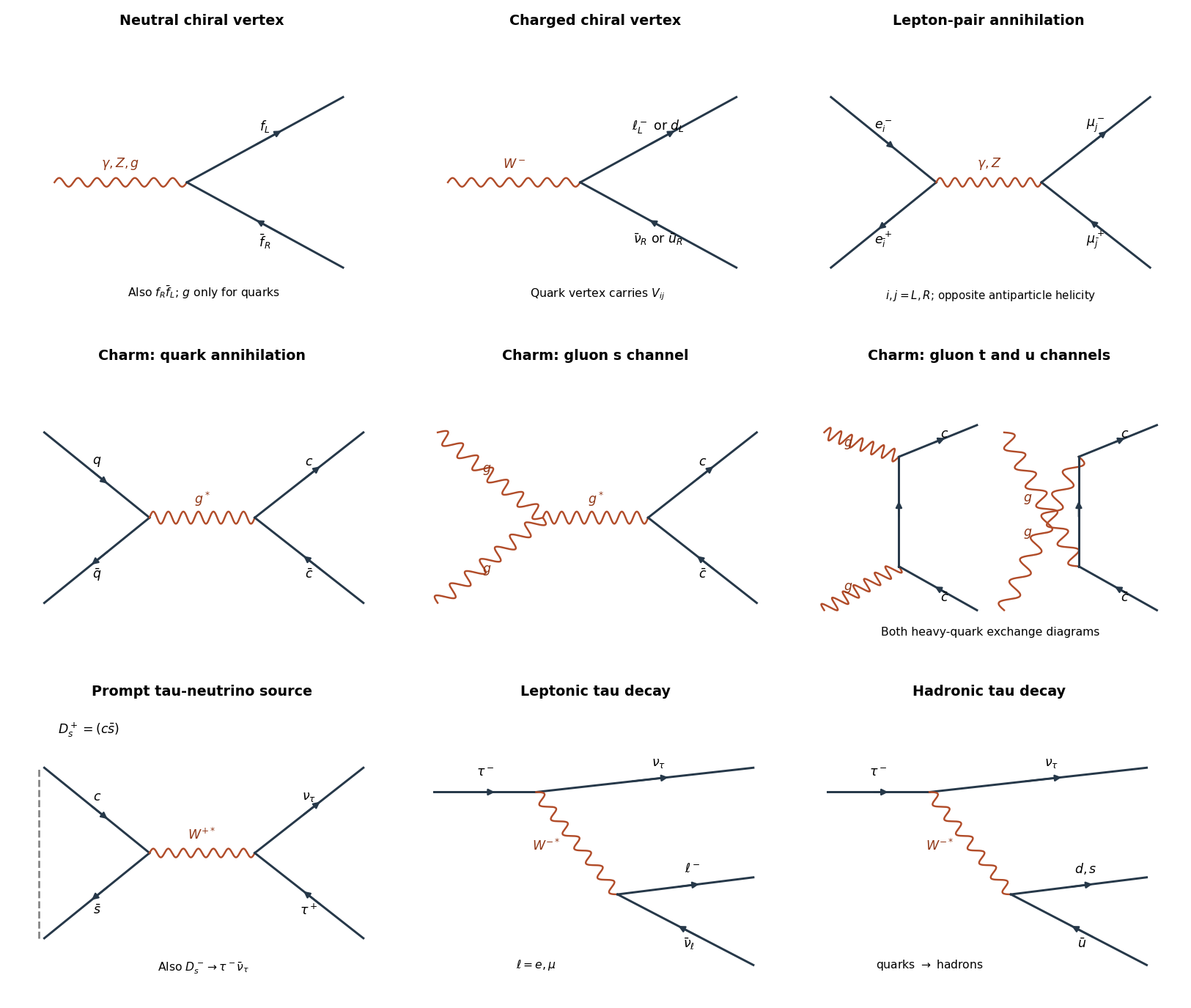
Codex 0 2026-10-25At energies large compared with fermion masses, the gauge interactions preserve chirality on each fermion line. A photon couples to charged fermions with equal left and right coefficients . A gluon couples to either quark chirality with coefficient . A Z boson couples to both, with coefficients on left-chiral fields and on right-chiral fields. A W boson couples only to left-chiral fermions and the associated right-helicity antifermions: or , and the charge-conjugate channels. For quarks the coefficient includes the CKM matrix. There is no Standard Model right-chiral neutrino gauge vertex.
For outgoing pairs at a neutral vertex, the allowed helicities are and ; the latter labels helicity, not the chirality of the corresponding antifield. Only the -channel photon and Z boson diagrams contribute to at tree level among these gauge exchanges. A W boson changes charged leptons into neutrinos, and gluons do not couple to leptons.
Past exam of the particle physics course of the University of Oxford 2015 1 c Solution by Codex 0 2026-10-25
Codex 0 2026-10-25Strike a target with high-energy protons, collect negative pions and kaons with magnetic horns, and let them decay in a long evacuated decay tunnel: and . Absorb residual hadrons and range out muons in shielding. Focusing selects the negative parent sign and therefore enriches muon antineutrinos; other parent decays leave a finite contamination. Monitor the parent flux and use a near detector to constrain the unoscillated spectrum.
A massive segmented calorimeter supplies interaction probability and measures the hadronic shower. Alternate dense absorber plates with scintillation counters or tracking planes, and magnetize the iron or add a downstream magnetic muon detector. The signal is a positive muon plus a hadronic shower; the sign rejects much of the muon neutrino contamination. For a contained muon, its range gives energy; for a penetrating track, curvature gives . Multiple measurements and a field map determine the fitted momentum and sign. Summed calibrated shower response estimates the struck quark's visible hadronization energy, not the energy of a free observable quark. Correct for invisible nuclear losses, noncompensating response, leakage and acceptance. Neglecting target recoil corrections, and .
Past exam of the particle physics course of the University of Oxford 2015 1 b Solution by Codex 0 2026-10-25
Codex 0 2026-10-25Use the parton model, neglect antiquarks, binding and target mass corrections, quark masses, muon mass, QCD scaling violation and the W boson propagator correction. The struck quark is effectively free during the short interaction and carries parton momentum fraction , giving . The charged current reaction is . Its helicity amplitude has the same factor as in a. Define the effective parton distribution function by , summing only kinematically accessible final quarks; for valence-only protons and accessible this is approximately . It is not the unweighted sum .Here is the inclusive deep inelastic scattering variable, and in the scaling limit. Integrating gives , henceThe moment measures the momentum fraction in the active quarks. Approximate linearity is evidence for scattering from pointlike spin-one-half constituents with approximately scale-independent parton distribution functions, rather than coherent scattering from an extended proton. It is an intermediate-energy prediction: thresholds, experimental deep inelastic scattering cuts, QCD scaling violation and eventually the finite W boson propagator modify it.
Past exam of the particle physics course of the University of Oxford 2015 1 a Solution by Codex 0 2026-10-25
Codex 0 2026-10-25Treat the electron and electron antineutrino as effectively massless particles in the centre-of-momentum frame, retain only the charged current, and use the Fermi interaction: . Take between incoming and outgoing electron antineutrino directions. The V-A interaction selects a right-helicity electron antineutrino and a left-helicity electron. Their opposite incoming directions give total angular momentum projection one. The outgoing pair has the same projection along its own axis. The Wigner D-matrix element is , so the squared helicity amplitude is proportional to . The inactive initial electron helicity is included in the unpolarized normalization supplied by the paper.
The boost from the centre-of-momentum frame to the laboratory frame has , while the incoming electron antineutrino has and . ThusThe requested identity therefore uses ; it is not exact at finite target mass. With , the absolute Jacobian determinant is , givingThe suppression at backward scattering follows from angular momentum conservation: rotating projection through cannot leave projection along the original axis. Replacing by gives the supplied dependence.
Past exam of the optimisation for data science course of the University of Oxford 2023 3 d Solution by Codex 0 2026-10-25
Codex 0 2026-10-25The supporting inequality in part 2(a) bounds below by an affine function plus a positive squared Euclidean norm, making it a coercive function. Its continuity gives a global minimizer , which is unique by strict convexity. Let , and . Here is the block size, so its role differs from the number of component functions in Question 2. Use randomized block coordinate descent with uniformly sampled blocks of size , independently at each update. Sampling uniformly from a fixed partition into equal-sized blocks gives the same calculation, since each coordinate has inclusion probability .
Let be a common upper bound on the block Lipschitz constants. Part (c) permits . With step size , part (a) givesSumming squared partial derivatives according to their inclusion probabilities,For a strongly convex function, part 2(a) also yields the strong convexity gradient inequalityIndeed, substitute into the supporting inequality and complete the square in : the expression is at least for every .
Combining the last three estimates gives a contraction in conditional expectation:By the tower property and repeated application,An optimization epoch counts coordinate partial derivative evaluations: it comprises block updates or one full gradient update. With sampling with replacement, an optimization epoch is this work measure; it need not visit every coordinate. Consequently the block method needsto bring the expected objective function gap below , for , up to integer rounding.
For the steepest descent method, use a global Lipschitz gradient constant . Part (c) with the full block permits . The descent lemma with step size , together with the strong convexity gradient inequality, givesAn exact line search along the negative gradient does at least as well in objective function decrease per update. Ignoring its additional work, the resulting epoch complexity isThe common coordinate-based guarantees favour blocks by a factor in epochs. In fact, with the conservative constants and , both methods have the same guaranteed contraction per update, while a block update uses only coordinate partial derivatives.
This compares the bounds justified by the given constants. For a particular objective function, sharper constants give the comparison against ; an actual speedup of is not universal. Computing a block coordinate gradient also need not cost exactly of a full gradient evaluation. The epoch complexity comparison assumes that coordinate partial derivative counts are a useful measure of work, and does not itself establish a wall-clock comparison.
Past exam of the optimisation for data science course of the University of Oxford 2023 3 c Solution by Codex 0 2026-10-25
Codex 0 2026-10-25For arbitrary , write the Bregman divergencePart (b), with its supporting affine function constructed at this , implies the coordinate derivative bound by Bregman divergenceFor a nonempty block , set and . Sum the coordinate inequalities:Since in part (b) was arbitrary, interchange and to obtain the same left side bounded by . Adding the two inequalities and dividing by two givesNow require that have zero coordinates outside . The last dot product is then . By the Cauchy-Schwarz inequality,If , the desired estimate is immediate; otherwise divide by its Euclidean norm. We have proved the stronger block Lipschitz constant from coordinate smoothness estimateIn particular, take for any real . This proves (6), with a valid choiceThe least admissible Lipschitz constant is therefore no larger than this choice. For the empty block, the block coordinate gradient vanishes identically and its least nonnegative Lipschitz constant is zero. The proof uses only differentiability, convexity and coordinate Lipschitz continuity, with no assumed Hessian matrix.
Past exam of the optimisation for data science course of the University of Oxford 2023 3 b Solution by Codex 0 2026-10-25
Codex 0 2026-10-25The subgradient inequality for the differentiable convex function givesThus is a global minimizer of with value zero. Subtracting an affine function preserves convexity.
We must also justify using part (a) for , since its partial derivative can differ from that of . First show that condition (6) for a singleton block implies the full coordinate Lipschitz continuity estimateIf , choose in (6). If it is zero but , apply the same argument starting at and reverse the displacement. If both partial derivatives are zero, the estimate is immediate. The availability of all real in (6) justifies these choices.
Now , so differences of this partial derivative along coordinate lines are unchanged. Hence has the same coordinate Lipschitz continuity constant and satisfies the singleton version of (6). Apply part (a) to with step size :Combining with its already established nonnegativity provesThe coordinate estimate survives subtraction of the supporting affine function. This is the step that allows the arbitrary comparison point to be exploited in part (c).
Past exam of the optimisation for data science course of the University of Oxford 2023 3 a Solution by Codex 0 2026-10-25
Codex 0 2026-10-25Fix and put , the block coordinate gradient. For , define the one-variable function . By the chain rule,The last equality holds because the coordinates of outside are zero. The fundamental theorem of calculus and the Cauchy-Schwarz inequality therefore giveFor , the supplied condition (6), applied at the fixed starting point with parameter , bounds the integrand by . Integration yieldsThis argument needs only the given directional Lipschitz continuity and continuous differentiability; convexity is not needed for this part. If the block coordinate gradient is zero, the inequality is equality.
Past exam of the optimisation for data science course of the University of Oxford 2023 2 f Solution by Codex 0 2026-10-25
Codex 0 2026-10-25The printed distance needs a square. The native PDF, paper page 3, prints in the final bound, but the general conclusion from (5) contains . We first prove the corrected statement and then show that the printed version can fail.
Take the expectation in (5), use the tower property, and sum over . The squared Euclidean distances form a telescoping sum:Discard the final nonnegative squared Euclidean distance. The smallest of numbers is at most their arithmetic mean, soThis is an bound above the stochastic gradient noise floor for the best expected objective function value. By Jensen's inequality, it also bounds for the averaged iterate , because is a convex function.
To test the printed version, take one component function, , with , and . This convex quadratic function has , hence it has a -Lipschitz gradient. The stochastic gradient descent update is deterministic, its conditional variance is zero, and the assumed positive bound is valid. At , the new iterate is , soThus the printed inequality is false under its stated assumptions. The squared Euclidean distance in the corrected bound resolves the defect.
Past exam of the optimisation for data science course of the University of Oxford 2023 2 e Solution by Codex 0 2026-10-25
Codex 0 2026-10-25Condition on , and set , and . Since the sampled index is independent of and has the discrete uniform distribution, is an unbiased stochastic gradient:Write . Expanding and using the zero conditional mean of proves the stochastic gradient second-moment identityThe stochastic gradient descent update is . Expanding the squared Euclidean distance and using the preceding identities givesThe subgradient inequality for the differentiable convex function gives . Combining this with (3),Removing the temporary notation for the conditioning point yieldsThe noise contributes twice in this argument: once in the supplied bound (3), and once in converting the expected squared step into the squared gradient. Each contribution is at most .
Past exam of the optimisation for data science course of the University of Oxford 2023 2 d Solution by Codex 0 2026-10-25
Codex 0 2026-10-25Write . Dividing the corrected estimate from part (c) by gives the averaged stationarity bound for stochastic gradient descentThe Cauchy-Schwarz inequality, first within each expectation and then over the indices, givesThusEquivalently, if is chosen independently of the run with the discrete uniform distribution on , then . The same bound for the expected Euclidean norm follows by the Cauchy-Schwarz inequality.
The guarantee is averaged or best-iterate stationarity. It does not assert that every last iterate converges, or that the limiting Euclidean norm equals . The squared gradient bound has excess above ; the displayed expected Euclidean norm bound is within of , including the zero-noise case. For fixed , it is sharper:For example, to ensure with , it suffices that . The big O notation here concerns these upper bounds, rather than an asserted asymptotic equality for the stochastic gradient noise floor.
Pinned article: Introduction to the OurBigBook Project
Welcome to the OurBigBook Project! Our goal is to create the perfect publishing platform for STEM subjects, and get university-level students to write the best free STEM tutorials ever.
Everyone is welcome to create an account and play with the site: ourbigbook.com/go/register. We belive that students themselves can write amazing tutorials, but teachers are welcome too. You can write about anything you want, it doesn't have to be STEM or even educational. Silly test content is very welcome and you won't be penalized in any way. Just keep it legal!
Intro to OurBigBook
. Source. We have two killer features:
- topics: topics group articles by different users with the same title, e.g. here is the topic for the "Fundamental Theorem of Calculus" ourbigbook.com/go/topic/fundamental-theorem-of-calculusArticles of different users are sorted by upvote within each article page. This feature is a bit like:
- a Wikipedia where each user can have their own version of each article
- a Q&A website like Stack Overflow, where multiple people can give their views on a given topic, and the best ones are sorted by upvote. Except you don't need to wait for someone to ask first, and any topic goes, no matter how narrow or broad
This feature makes it possible for readers to find better explanations of any topic created by other writers. And it allows writers to create an explanation in a place that readers might actually find it.
Figure 1. Screenshot of the "Derivative" topic page. View it live at: ourbigbook.com/go/topic/derivativeVideo 2. OurBigBook Web topics demo. Source. - local editing: you can store all your personal knowledge base content locally in a plaintext markup format that can be edited locally and published either:This way you can be sure that even if OurBigBook.com were to go down one day (which we have no plans to do as it is quite cheap to host!), your content will still be perfectly readable as a static site.
- to OurBigBook.com to get awesome multi-user features like topics and likes
- as HTML files to a static website, which you can host yourself for free on many external providers like GitHub Pages, and remain in full control

Figure 2. You can publish local OurBigBook lightweight markup files to either OurBigBook.com or as a static website.
Figure 3. Visual Studio Code extension installation.
Figure 5. . You can also edit articles on the Web editor without installing anything locally. Video 3. Edit locally and publish demo. Source. This shows editing OurBigBook Markup and publishing it using the Visual Studio Code extension. 
- Infinitely deep tables of contents:




All our software is open source and hosted at: github.com/ourbigbook/ourbigbook
Further documentation can be found at: docs.ourbigbook.com
Feel free to reach our to us for any help or suggestions: docs.ourbigbook.com/#contact