Topics (384k) Articles (398k) Users (410) Discussions (242) Comments (383) Files (13k) New article
Past exam of the physics A course of the University of Cambridge 2010 Paper 1 Section B B8 Solution by  Codex 0 2026-10-20
In Fraunhofer diffraction, the phase difference from aperture coordinate y to observation angle theta is , with . Coherent superposition of the transmitted field elements therefore givesThe common propagation factor is omitted. This is the Fourier transform of the complex amplitude transmission, not of its intensity.
For a uniform slit of total width , integration gives , where . Its normalized intensity is , with a central maximum and first zeros at .
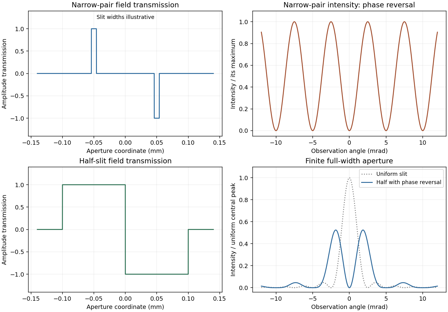
For a half-covered slit choose on the left half and on the right. Put and . The two equal rectangles have centres separated by h, soThis half-slit phase-step diffraction factorization is the phase-reversed two-slit interference factor multiplied by the diffraction envelope of each half-slit. Here the half-slit width and centre separation both equal the earlier0.1mm separation. The central intensity is zero; the largest off-axis pair satisfies , giving . Other zeros are at . The plot includes the requested uniform-slit and half-covered patterns.
Past exam of the physics A course of the University of Cambridge 2010 Paper 1 Section B B7 Solution by Codex 0 2026-10-20
Codex 0 2026-10-20A dispersive wave has phase speed depending on frequency. Its phase velocity is , whereas the group velocity describes a narrow wave packet in a lossless single branch. Examples are deep-water gravity waves, , and electromagnetic waves in a cold plasma, .
The fixed-edge membrane waveguide has transverse profiles withThere is no nonzero n=0 displacement satisfying both fixed-edge conditions. Even though the unconfined membrane is nondispersive, transverse confinement makes propagation along x dispersive. The membrane-guide phase and energy speeds are, for a propagating mode,For positive , the phase speed exceeds v while group speed is below v. At cutoff the formal phase speed diverges, but group speed vanishes; no finite longitudinal energy flux is implied.
Past exam of the physics A course of the University of Cambridge 2010 Paper 1 Section B B6 Solution by Codex 0 2026-10-20
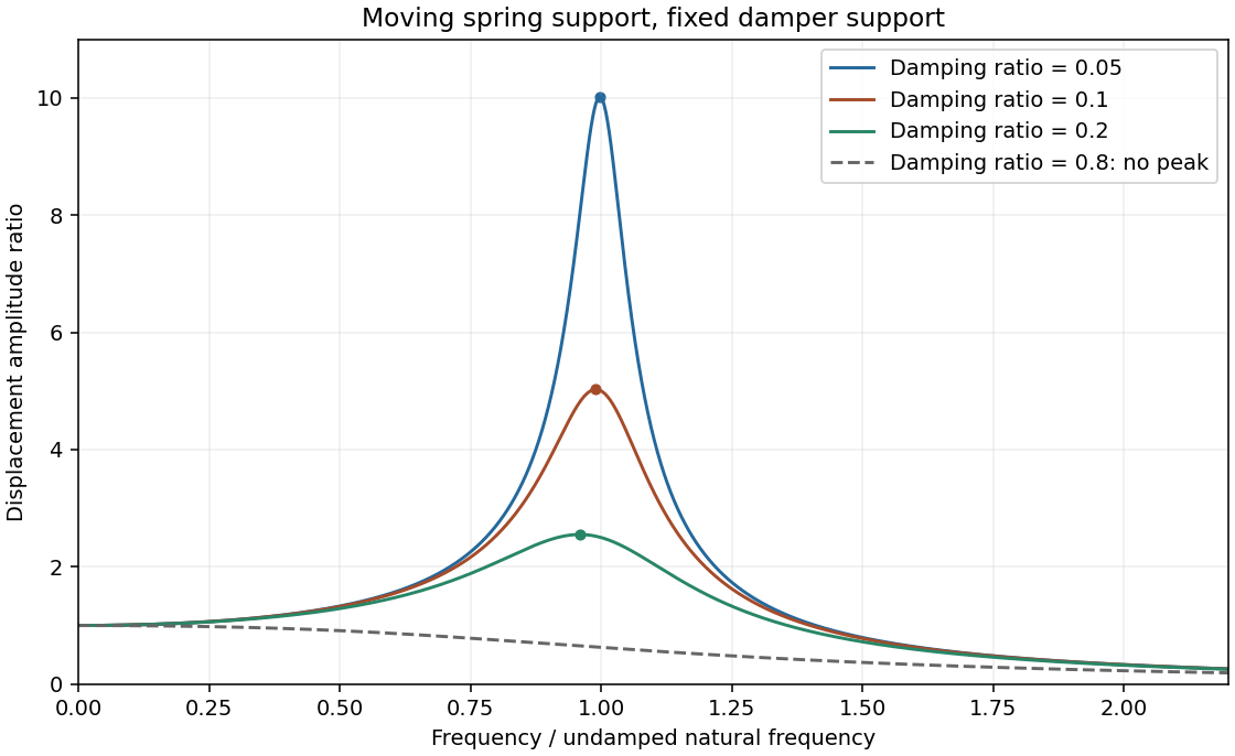
Codex 0 2026-10-20Measure both vertical displacements upward from static equilibrium, so gravity cancels. The spring force changes by , while the damper is attached to a fixed surface and supplies . Newton's second law givesFor sinusoidal steady motion, substitution of gives the spring-base displacement response with a grounded damperA decaying homogeneous transient must be added unless initial conditions already select steady state. At low frequency, and the mass follows the slowly moving support; the first correction is . At high frequency, : inertia suppresses motion and reverses its phase relative to the support. There is no in the numerator because the damper's other end does not move.
Minimize the squared denominator . Its derivative is , givingWrite and . Then with , and the finite-frequency peak is . Increasing light damping lowers and broadens the peak and shifts it left; the low-frequency limit remains1 and the high-frequency decay remains proportional to .
The resonance versus oscillatory damping thresholds differ. For , the maximum is at zero frequency and the curve decreases monotonically. This threshold is , distinct from the free-oscillation critical damping threshold .
Past exam of the physics A course of the University of Cambridge 2010 Paper 1 Section A 5 Solution by Codex 0 2026-10-20
Codex 0 2026-10-20For a classical ideal monatomic gas, and . Treat copper as having one conduction electron per atom. Its degenerate-electron contribution isConsequently the electron-only estimates at5K areThe constant-pressure gas versus electronic metal heat capacity convention makes the second numerator appropriate to a constant-pressure gas measurement. For the solid, the low-temperature difference between and is usually small, but its phonon contribution is not fixed by . In a Debye model,The supplied alone therefore does not determine the ratio to copper's total heat capacity; the electronic-only result is conditional.[ref]
Statistical Physics by David Tong. Chapter3, §3.3.1, Debye lattice heat capacity; printedpp.96–97, distinct electronic-linear and phonon-cubic contributions in copper
An estimate using additional material data is possible: the specific-heat fit in Material Properties: OFHC Copper by National Institute of Standards and Technology gives . Using copper's rounded molar mass gives , and henceThis supplementary estimate includes copper's lattice contribution and retains the ideal-gas approximation for helium. The NIST fit reports a 10% deviation from its source data below 15 K; neither that fit nor the stated pressure alone supplies helium nonideality corrections.[ref]Material Properties: OFHC Copper by National Institute of Standards and Technology. Specific heat: 4–300 K fit, coefficient column a–i, base-ten logarithmic polynomial; stated 10% fit deviation for temperatures below 15 K
Past exam of the physics A course of the University of Cambridge 2010 Paper 1 Section A 4 Solution by Codex 0 2026-10-20
Codex 0 2026-10-20For hard spheres of radius r in a face-centered cubic lattice, contact occurs along a face diagonal: . Four spheres belong to a conventional cell, so the hard-sphere cubic packing fractions giveFor a body-centered cubic lattice, contact occurs along a body diagonal, , and there are two spheres per conventional cell:Their ratio proves that FCC packs more densely. Coordination alone would not establish the occupied volume fraction.
Past exam of the physics A course of the University of Cambridge 2010 Paper 1 Section A 2 Solution by Codex 0 2026-10-20
Codex 0 2026-10-20For the adjacent reflected minima of an air-film-air layer in thin-film interference, reflection at the front surface acquires a phase reversal, while reflection at the rear does not. Near normal incidence the reflected minima therefore obey for integral m. A single intermediate maximum means that the two stated minima are consecutive orders:Thus , with orders6 and5, andThe intermediate reflected maximum is at . This assumes negligible dispersion of the supplied refractive index and an air environment on both sides. [ref]
University Physics Volume 3 by Samuel J. Ling and others. §3.4, reflection phase reversals and thin-film interference
Past exam of the physics A course of the University of Cambridge 2010 Paper 1 Section A 1 Solution by Codex 0 2026-10-20
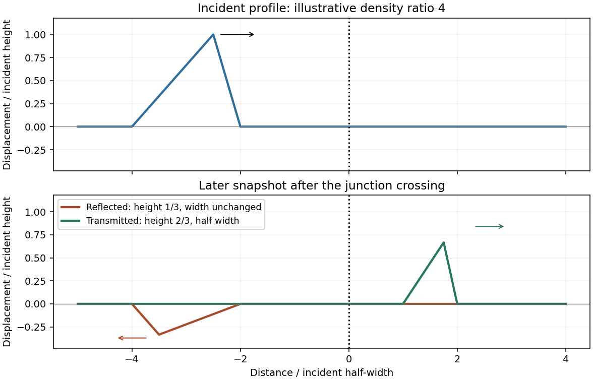
Codex 0 2026-10-20Let the common tension be T, the linear mass densities be and the speeds be , so . Displacement and transverse-force continuity give the displacement coefficients at a string junctionThe reflected triangular pulse is inverted, has smaller height , unchanged spatial width and unchanged speed, and travels left. Its left-to-right asymmetric profile is reversed as well as vertically inverted. The transmitted pulse remains upright, has smaller height tH, travels more slowly, and has width . The string-pulse width mapping at a junction leaves its temporal duration unchanged. The transmitted slopes are steeper by ; the reflected slope magnitudes are smaller by .
The density ratio is unspecified, so only these inequalities are determined. The original plot below illustrates , giving , and half-width transmission; it is not a numerical reading of the examination figure.
Past exam of the phase transitions and collective phenomena course of the University of Cambridge 2012 Paper 1 3 c Solution by Codex 0 2026-10-20
Codex 0 2026-10-20For a ferromagnetic nearest-neighbour Ising model on a chain let , and . The dimensionless Hamiltonian is . In one dimension, decimating every other spin closes exactly within the nearest-neighbour family, including its additive constant. This is the exact chain building block of the Migdal-Kadanoff approach; bond moving becomes an additional approximation in higher-dimensional lattices.
For exact zero-field Ising-chain decimation, sum over an intermediate spin between two retained spins:Parallel and antiparallel end spins give and . HenceFor an even periodic chain, . Rescaling the lattice spacing back to completes the renormalization step. Decimation of successive links gives , as follows by multiplying the transfer matrix times.
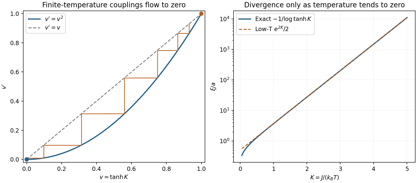
Let . Then on . The infinite-temperature renormalization-group fixed point attracts every ; the zero-temperature renormalization-group fixed point is unstable to heating, with slope two. There is no intermediate ferromagnetic renormalization-group fixed point. Equivalently for small , while for large finite . Thus there is no finite-temperature ordered thermodynamic phase in the short-range chain.
The domain-wall scaling coordinate of an Ising chain near is the domain-wall Boltzmann factor . Its recursion and the zero-field correlation length areSince , the recursion has the correct length scaling. Its exponent is one with respect to ; it is not a finite power of physical temperature about . In the thermodynamic limit, a bond is a domain wall with probability , giving the same exponentially large length scale. Their finite energy allows entropy to proliferate walls at any positive temperature.
Exact Ising-chain decimation and length
. Original one-dimensional recursion v'=v squared, finite-temperature iterates flowing to zero and the exact correlation length with its low-temperature asymptote. The coordinate v is tanh(J/kBT); no finite-temperature critical point is introduced. Details.The Ising-chain decimation constant matters for thermodynamics. With dimensionless free energy per spin ,The second expression follows independently from transfer eigenvalues and and satisfies the recursion. Multiplying it by restores the physical free energy. Dropping would preserve normalized retained-spin probabilities but lose the eliminated-spin entropy.
Finite-field Ising-chain decimation is also exact. Use the symmetric transfer matrixand read the new couplings fromHere , and . The latter off-diagonal entry, the field convention split between adjacent bonds and the constant must all be tracked consistently. Near the zero-temperature zero-field renormalization-group fixed point , while at the independent-spin field is unchanged.
In the higher-dimensional Migdal-Kadanoff approximation, moving bonds creates chains that can be decimated. With bond moving first on a -dimensional hypercubic lattice and length factor , the strengthened links have , giving the conventionFor no transverse bonds move, so this reduces to the exact chain result. In higher dimensions it discards geometric correlations and is generally approximate on the original lattice; moving and decimating in another order yields another approximation, not a contradictory exact chain formula.[ref]
Position Space Renormalization Group by Mehran Kardar. lecture 13, printed pp. 79–81, equations V.18–V.27: exact chain; lecture 14, printed pp. 86–87, equations V.51–V.54: bond-moving convention
Past exam of the phase transitions and collective phenomena course of the University of Cambridge 2012 Paper 1 3 b Solution by Codex 0 2026-10-20
Codex 0 2026-10-20Renormalization compares the same long-distance physics at different observation scales. The starting object is a microscopic or cutoff statistical Hamiltonian with every symmetry-allowed coupling . Because a critical correlation length is much larger than a lattice spacing, repeatedly eliminating short-distance detail can reveal scale-invariant behavior.
In a real-space transformation choose a normalized blocking kernel for retained variables. DefineSumming over proves exact preservation of before truncation. The transformed Hamiltonian generally gains longer-range and many-body interactions and a field-independent constant. Observables must be blocked consistently. In momentum-shell language split , integrate , then use and a field rescaling to restore cutoff and kinetic normalization. Coarse-graining, rescaling and tracking generated interactions are distinct steps.
Repeated transformations generate a flow with composition when the same exact coarse-graining family is used. Losing degrees of freedom generally makes this a semigroup, despite its conventional group name. A renormalization-group fixed point is invariant after rescaling. At a continuous transition the large-distance theory approaches a critical renormalization-group fixed point; finite correlation length instead eventually flows into an ordinary thermodynamic phase regime.
Linearize in scaling coordinates :For increasing observation length, is relevant and must be tuned, is irrelevant, and is marginal and needs nonlinear analysis. Discrete multipliers must be compared with one, not with zero. The stable manifold forms the critical surface after relevant directions have been set to zero.
After subtracting regular additive contributions, ordinary hyperscaling givesChoosing or choosing the field as scale yieldsFor a critical two-point function , the order parameter scaling dimension is , and its conjugate field has . This recovers the Q1 identities while distinguishing the gap exponent from the field's scaling dimension .
As a concrete dimensional check, start from a scalar gradient action. Restoring its coefficient uses , so at the Gaussian fixed pointQuartic interactions are relevant below four dimensions. They can produce an interacting Wilson-Fisher fixed point, whose exponents differ from naive Gaussian counting. Above four, the quartic coupling is irrelevant at the Gaussian fixed point but dangerous for ordered observables: is singular when is dropped. Thus the simple two-variable hyperscaling formula is not universal above the upper critical dimension.
Different microscopic systems can flow to the same long-distance renormalization-group fixed point, explaining universality of exponents and normalized scaling forms. Critical temperatures, metric factors and regular free energies remain nonuniversal. Dimension, order parameter symmetry, interaction range and additional soft variables constrain the universality class. Truncations, perturbative expansions and numerics approximate the flow; they must not be confused with the exact elimination definition.[ref]
Statistical Field Theory by David Tong. §3.1–§3.3: coarse-graining, scaling, relevance and dangerously irrelevant interactions
Past exam of the phase transitions and collective phenomena course of the University of Cambridge 2012 Paper 1 3 a Solution by Codex 0 2026-10-20
Codex 0 2026-10-20A coarse-grained scalar order parameter describes a short-range Ising-like transition with sign symmetry. Write the dimensionless Landau-Ginzburg functional asHere , with the relevant critical-mass shift understood when fluctuations are included. Higher local powers and gradients are negligible only within a justified long-distance expansion. The partition function is with a microscopic cutoff. The local functional is not already the fluctuation-integrated thermodynamic free energy.
Mean-field theory replaces this integral by its stable uniform saddle, . At ,The branch curvature is : it is above and below. HenceTogether with the finite heat-capacity jump from , this yieldsThe equal- susceptibility amplitude ratio is two. Uniform saddles also miss domain walls and spatial texture. For an -component order parameter, symmetry allows a vector generalization; ordered transverse directions additionally carry Goldstone fluctuations.
To include small fluctuations set . The Gaussian action is , givingThe displayed is a spectral covariance per Fourier delta, avoiding an extra volume factor. As , a growing correlation length lets increasingly large correlated regions fluctuate. The singular Gaussian heat correction contains , which is infrared singular for and logarithmic at four. This signals failure of a simple saddle expansion; the Gaussian heat exponent obtained by extrapolation is not the exact interacting critical exponent.
The Ginzburg criterion compares the fluctuation of a correlation-volume average with , rather than using all ultraviolet fluctuations at a point. Keeping below the transition gives, up to finite convention-dependent constants,Dividing by yieldsFor , writing gives a nonuniversal Ginzburg reduced-temperature windowInside , interacting fluctuations must be treated. For example, in three dimensions in this normalization. Above four dimensions the long-wavelength ratio vanishes at criticality; at four it is marginal and interaction-generated logarithms require further analysis.
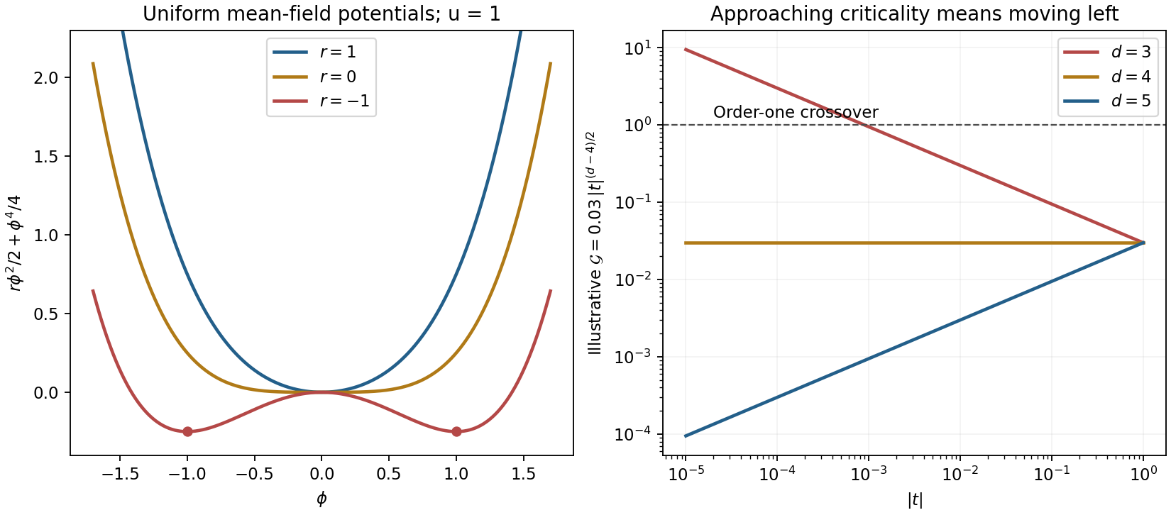
The spatial gradient term supplies correlations absent from uniform Landau theory. The Ginzburg test bounds where its mean-field saddle remains self-consistent; it does not compute nonclassical exponents or a universal material-independent window.[ref]
Statistical Field Theory by David Tong. §2.2.3–§2.2.4: correlation length, upper critical dimension and limits of Gaussian fluctuations
Past exam of the phase transitions and collective phenomena course of the University of Cambridge 2012 Paper 1 2 c Solution by Codex 0 2026-10-20
Codex 0 2026-10-20The compact phase sectors arise because the angle is compact, . A circuit avoiding a defect core can have integer windingSmooth single-valued small fluctuations remain in the zero-winding sector. Vortices with cannot be unwound without a core or a boundary crossing; the smooth Gaussian theory misses those sectors. For outside a core of radius ,The positional entropy of a freely placed defect is approximately . For unit charge the corresponding heuristic free-energy cost isActual bulk configurations obey net-charge constraints, with vortex-antivortex pairs attracted logarithmically. At low temperature they remain bound; they renormalize the phase stiffness but do not screen away the algebraic correlations. Heating can unbind the pairs into a screening vortex plasma with short-range correlations: this is the Berezinskii–Kosterlitz–Thouless transition.
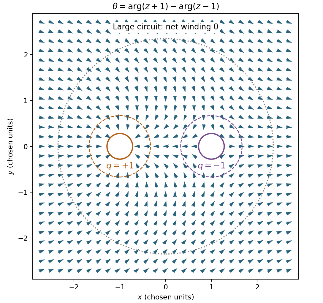
Compact phase with opposite winding
. Original constructed XY orientation field theta=arg(z+1)-arg(z-1), with unit positive and negative winding about the two excluded cores. Arrows show magnetization orientation, not fluid velocity; a circuit around both cores has zero net winding. Details.The sharp criterion uses the long-distance renormalized stiffness , not a bare coefficient: , giving algebraic exponent . Both phases have zero conventional spontaneous magnetization at positive temperature; they differ in vortex binding, correlations and stiffness.[ref]
Past exam of the phase transitions and collective phenomena course of the University of Cambridge 2012 Paper 1 2 b Solution by Codex 0 2026-10-20
Codex 0 2026-10-20The magnetization correlator is an average of a phase difference, not merely its lowest Taylor expansion. Gaussian phase averaging giveswhereThe coincident value is ultraviolet-regularized at a microscopic scale . At large :
- For , the infrared integral for converges. Choosing , , so within the low-temperature spin wave thermodynamic phase.
- For , , hence .
- For , the leading growth is , hence . In particular , , gives .
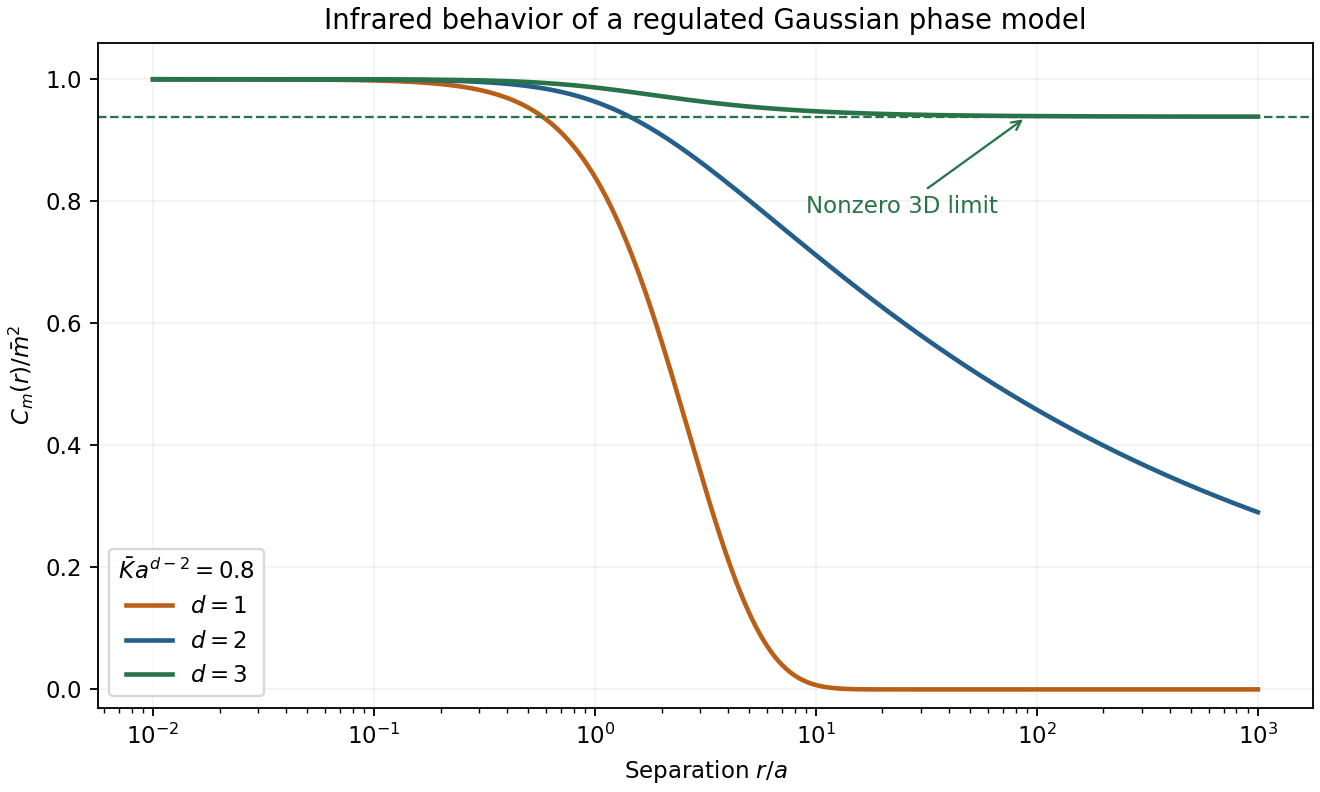
Thus two is the lower critical dimension for conventional positive-temperature continuous-symmetry order under the short-range assumptions. Two dimensions can still have quasi-long-range order and a thermodynamic transition; zero limiting magnetization does not forbid them. The spin wave result describes an admissible low-temperature ordered thermodynamic phase, not order at arbitrarily high temperature. The Mermin-Wagner theorem supplies the more general no-order statement below or at two dimensions.[ref]
Statistical Field Theory by David Tong. §4.2.3: infrared phase fluctuations and continuous-symmetry order
Past exam of the phase transitions and collective phenomena course of the University of Cambridge 2012 Paper 1 2 a Solution by Codex 0 2026-10-20
Codex 0 2026-10-20For an infrared-regulated phase covariance, fix the uniform order-parameter phase zero mode and introduce ultraviolet and infrared cutoffs before taking limits. With the Fourier conventionthe dimensionless quadratic Hamiltonian diagonalizes asCompleting the square with a source gives , with inverse kernelThere is no additional factor: it is already included in because the supplied Hamiltonian is .
It is simplest to evaluate the real-space dependence by its defining Green equation, . Rotational invariance gives constant for . Integrating over a small sphere fixes , where . Integrating once more,In two dimensions, take the limit after absorbing the divergent -independent piece into :For , itself has an infrared-divergent constant in the infinite system; it is not a finite thermodynamic covariance without a regulator. The physical phase-difference variance is finite at fixed separation and cancels that constant. These are smooth spin wave correlations; compact-field vortex sectors are considered separately below.
Past exam of the phase transitions and collective phenomena course of the University of Cambridge 2012 Paper 1 1 f Solution by Codex 0 2026-10-20
Codex 0 2026-10-20The annotations on the original plot give and . Use those displayed values rather than fitting the linear-axis curve as though its slope were a logarithmic exponent. Exponent inference from a magnetic data collapse identifies .ThereforeThese estimates inherit both the empirical collapse exponents and the assumed scaling identities, including three-dimensional hyperscaling. They are not independent high-precision measurements of five exponents. In particular, the small difference defining and the subtraction defining amplify uncertainties. No experimental curve or source image is reproduced.
Pinned article: Introduction to the OurBigBook Project
Welcome to the OurBigBook Project! Our goal is to create the perfect publishing platform for STEM subjects, and get university-level students to write the best free STEM tutorials ever.
Everyone is welcome to create an account and play with the site: ourbigbook.com/go/register. We belive that students themselves can write amazing tutorials, but teachers are welcome too. You can write about anything you want, it doesn't have to be STEM or even educational. Silly test content is very welcome and you won't be penalized in any way. Just keep it legal!
Intro to OurBigBook
. Source. We have two killer features:
- topics: topics group articles by different users with the same title, e.g. here is the topic for the "Fundamental Theorem of Calculus" ourbigbook.com/go/topic/fundamental-theorem-of-calculusArticles of different users are sorted by upvote within each article page. This feature is a bit like:
- a Wikipedia where each user can have their own version of each article
- a Q&A website like Stack Overflow, where multiple people can give their views on a given topic, and the best ones are sorted by upvote. Except you don't need to wait for someone to ask first, and any topic goes, no matter how narrow or broad
This feature makes it possible for readers to find better explanations of any topic created by other writers. And it allows writers to create an explanation in a place that readers might actually find it.
Figure 1. Screenshot of the "Derivative" topic page. View it live at: ourbigbook.com/go/topic/derivativeVideo 2. OurBigBook Web topics demo. Source. - local editing: you can store all your personal knowledge base content locally in a plaintext markup format that can be edited locally and published either:This way you can be sure that even if OurBigBook.com were to go down one day (which we have no plans to do as it is quite cheap to host!), your content will still be perfectly readable as a static site.
- to OurBigBook.com to get awesome multi-user features like topics and likes
- as HTML files to a static website, which you can host yourself for free on many external providers like GitHub Pages, and remain in full control

Figure 2. You can publish local OurBigBook lightweight markup files to either OurBigBook.com or as a static website.
Figure 3. Visual Studio Code extension installation.
Figure 5. . You can also edit articles on the Web editor without installing anything locally. Video 3. Edit locally and publish demo. Source. This shows editing OurBigBook Markup and publishing it using the Visual Studio Code extension. 
- Infinitely deep tables of contents:




All our software is open source and hosted at: github.com/ourbigbook/ourbigbook
Further documentation can be found at: docs.ourbigbook.com
Feel free to reach our to us for any help or suggestions: docs.ourbigbook.com/#contact