Topics (384k) Articles (398k) Users (410) Discussions (242) Comments (383) Files (13k) New article
Past exam of the physics A course of the University of Cambridge 2011 Paper 2 Section D D13 Solution by  Codex 0 2026-10-20
An ideal operational amplifier draws no current at either input. With stable operational-amplifier negative feedback in its unsaturated linear range, infinite open-loop gain also gives a virtual short, . The amplifier adjusts its output to enforce that equality; it is not a conducting connection between the inputs. Here , so the ideal summing node is a virtual ground. Kirchhoff's current law gives , hence the ideal gain is .
For the finite-input-resistance inverting amplifier let the inverting-node voltage be , and continue to neglect output impedance. The controlled output and node-current balance areEliminating givesDividing the denominator by gives the requested resistance-sum form. The ideal result follows whenever ; taking alone is insufficient if is small. At finite frequency and the gain are phasor ratios, subject to feedback stability.
With equal resistors and sufficiently large loop gain, . This gives a controlled sign reversal or 180-degree phase inversion, useful for subtraction and opposite-phase signal paths, with amplitude set by a resistor ratio rather than uncertain open-loop gain. The source still sees approximately , so this is not a high-input-impedance voltage follower. For the ideal-input, single-pole model, the noise gain of an operational amplifier is two and the closed-loop bandwidth is approximately half the gain-bandwidth product. Output swing, slew rate and load constraints must also permit linear operation.
Past exam of the physics A course of the University of Cambridge 2011 Paper 2 Section C C10 Solution by Codex 0 2026-10-20
Codex 0 2026-10-20identical particles have the same intrinsic properties. Exchanging their bookkeeping labels cannot distinguish a physical preparation or change a measurable prediction. This is stronger than merely failing to track classical trajectories. For ordinary bosons and fermions, the many-particle wavefunction has respectively bosonic exchange symmetry or fermionic exchange symmetry under every particle exchange operator, acting on spatial and spin coordinates together. The Spin-statistics theorem connects integer spin to bosons and half-integer spin to fermions; this connection uses relativistic quantum-field assumptions, rather than following from the nonrelativistic Schrödinger equation alone.
For one-particle states satisfying orthonormality, the two alternatives form a quantum superposition:Its probability density contains an exchange interference term, absent from an incoherent mixture of labelled alternatives. The antisymmetric expression vanishes when both one-particle states are identical: one complete one-particle state can contain at most one fermion. This Pauli exclusion principle explains electron shell filling, the electronic Fermi sea and degeneracy pressure. Opposite spins are different one-particle states, so two electrons may share an atomic orbital. Spatially separated wave packets with negligible overlap can often be treated as distinguishable for local measurements; the underlying exchange symmetry remains.
In thermal equilibrium, occupation of a level of energy obeysbosons can accumulate macroscopically in one state, giving Bose-Einstein condensation; fermions instead fill successive states up to the Fermi energy at zero temperature. When occupation is dilute, both expressions reduce to the Maxwell-Boltzmann distribution. The identical-particle classical partition function contains , avoiding spurious entropy from permutations and the Gibbs paradox. Exchange effects become conspicuous when the thermal de Broglie wavelength is comparable to the interparticle spacing.
An operational test is the Hong-Ou-Mandel effect. Down-converted photon pairs enter separate ports of a balanced beam splitter; indistinguishable alternatives for one photon per output cancel. Scanning the relative arrival delay restores coincidences away from overlap. Matching polarization, spectral filtering and spatial alignment controls distinguishability; measuring delayed accidental coincidences controls background. The observed dip tests two-photon interference, and its finite depth must not automatically be interpreted as a failure of bosonic symmetry. The original apparatus varied beam-splitter position and subtracted a separately measured accidental background.[ref]
Measurement of Subpicosecond Time Intervals between Two Photons by Interference by C. K. Hong and others. pp. 2044–2046, Fig. 1, Eq. (2), coincidence-background procedure and Fig. 2
Past exam of the physics A course of the University of Cambridge 2011 Paper 2 Section B B9 Solution by Codex 0 2026-10-20
Codex 0 2026-10-20Put . Substitution of into the time-independent Schrödinger equation, followed by division by and multiplication by , separates the angular dependence:Thus andThe single-valued wavefunction condition, , requires . The regular boundary condition at the origin selects . Accordingly use in the radial ansatz; the printed notation describes the representatives.
For the two-dimensional Coulomb bound state, substitution of with the stipulated radial and energy scales givesThe coefficient of in the power series isThe regular solution otherwise has an exponentially growing contribution at large , incompatible with being normalizable. Termination at degree therefore requiresThe resulting is proportional to a Generalized Laguerre polynomial.
Define , the hydrogenic Rydberg energy for the stipulated mass. The first three distinct two-dimensional energies are , whereas in three dimensions they are . Both series approach zero from below, but the planar ground state is four times more tightly bound. Without spin the respective quantum degeneracies are and ; if individual degenerate states are counted, the second and third planar states already share the first excited energy. This comparison retains the supplied interaction; it does not replace it by the logarithmic electrostatic potential of a genuinely two-dimensional electromagnetic theory.
Past exam of the physics A course of the University of Cambridge 2011 Paper 2 Section B B8 Solution by Codex 0 2026-10-20
Codex 0 2026-10-20Write , retaining the printed magnetic moment convention. The displayed two-dimensional matrices are Pauli matrices, and the spin Hamiltonian operator isFor an x-directed field let . The Schrödinger equation gives and . With , these equations yieldEquivalently, . If denotes a positive elementary charge magnitude, a free electron is conventionally assigned a minus sign in its magnetic moment; that alternative reverses the rotation sense. The expressions here consistently use the moment specified in the paper.
Past exam of the physics A course of the University of Cambridge 2011 Paper 2 Section B B7 Solution by Codex 0 2026-10-20
Codex 0 2026-10-20A pure stationary state of a time-independent Hamiltonian operator is . Its probability density and all expectations of time-independent observables are constant. This does not require zero probability current.
For real scalar potential energy and no vector potential, substitute and its complex conjugate into . The potential terms cancel:Thus the probability current is . In a stationary state : flow may circulate without changing the density.
Here only the azimuthal phase contributes an imaginary logarithmic derivative. Since ,There is no radial or polar flow; the azimuthal current is independent of , so its divergence vanishes. The apparent coordinate singularity at cancels in the final expression.
The z-component of orbital angular momentum follows from the moment of the mass current:Indeed . This agrees with acting on the wavefunction.
Past exam of the physics A course of the University of Cambridge 2011 Paper 2 Section B B6 Solution by Codex 0 2026-10-20
Codex 0 2026-10-20For each mode in Cartesian coordinates, and . Consequently the two-dimensional isotropic harmonic oscillator hasThe normalized actions of the creation and annihilation operators areInvert their definitions as and , and similarly for . linear operators belonging to different coordinates commute, so substitution into givesEach term transfers one excitation between the two modes: , and likewise for its adjoint. Thus and, with no explicit time dependence, . This is conservation of angular momentum under planar rotations.
Finally and . HenceThe angular momentum is ; division by performs wavefunction normalization on this state without changing its eigenvalue. It is one excitation of the positive circular mode.
Past exam of the physics A course of the University of Cambridge 2011 Paper 2 Section A 5 Solution by Codex 0 2026-10-20
Codex 0 2026-10-20In the high-resolution quantization approximation, a smooth input distribution varies little across one conversion interval, so rounding to the nearest level gives an approximately uniform quantization error . ThereforeThe input must stay within the analogue-to-digital converter's range. A large standard deviation alone does not guarantee uniform quantization error: an input concentrated exactly on widely separated conversion levels has zero error. Truncation without a half-step correction also has a different mean and root mean square.
Past exam of the physics A course of the University of Cambridge 2011 Paper 2 Section A 4 Solution by Codex 0 2026-10-20
Codex 0 2026-10-20The central estimate is . propagation of uncertainty must include the occurrence of in both numerator and denominator. With angular derivatives measured per radian,Interpreting the two quoted errors as independent standard deviations, convert them to radians before calculatingIf the quoted errors are instead absolute bounds, the first-order worst-case estimate is . Correlated errors add to the variance. Treating and as independent would lose their shared measurement uncertainty.
Past exam of the physics A course of the University of Cambridge 2011 Paper 2 Section A 3 Solution by Codex 0 2026-10-20
Codex 0 2026-10-20The canonical commutation relation is . Applying the commutator product rule on a common operator domain,Equivalently, applying both sides to a twice differentiable test function gives , the same result.
Past exam of the physics A course of the University of Cambridge 2011 Paper 2 Section A 2 Solution by Codex 0 2026-10-20
Codex 0 2026-10-20The Sturm oscillation theorem gives three nodes of a wavefunction for the fourth bound state. reflection symmetry and nondegeneracy of one-dimensional bound states make it odd: one node of a wavefunction is at the centre, and the other two lie at opposite positions. In each flat allowed region the wavefunction is a sinusoid, with ; its wavelength is shortest in the central, deepest region. Outside the well it decays exponentially, with opposite signs on the two sides. Both and remain continuous at every finite step, as required by wavefunction matching at a finite potential step; only the curvature jumps. In particular, the wavefunction need not vanish at a step.
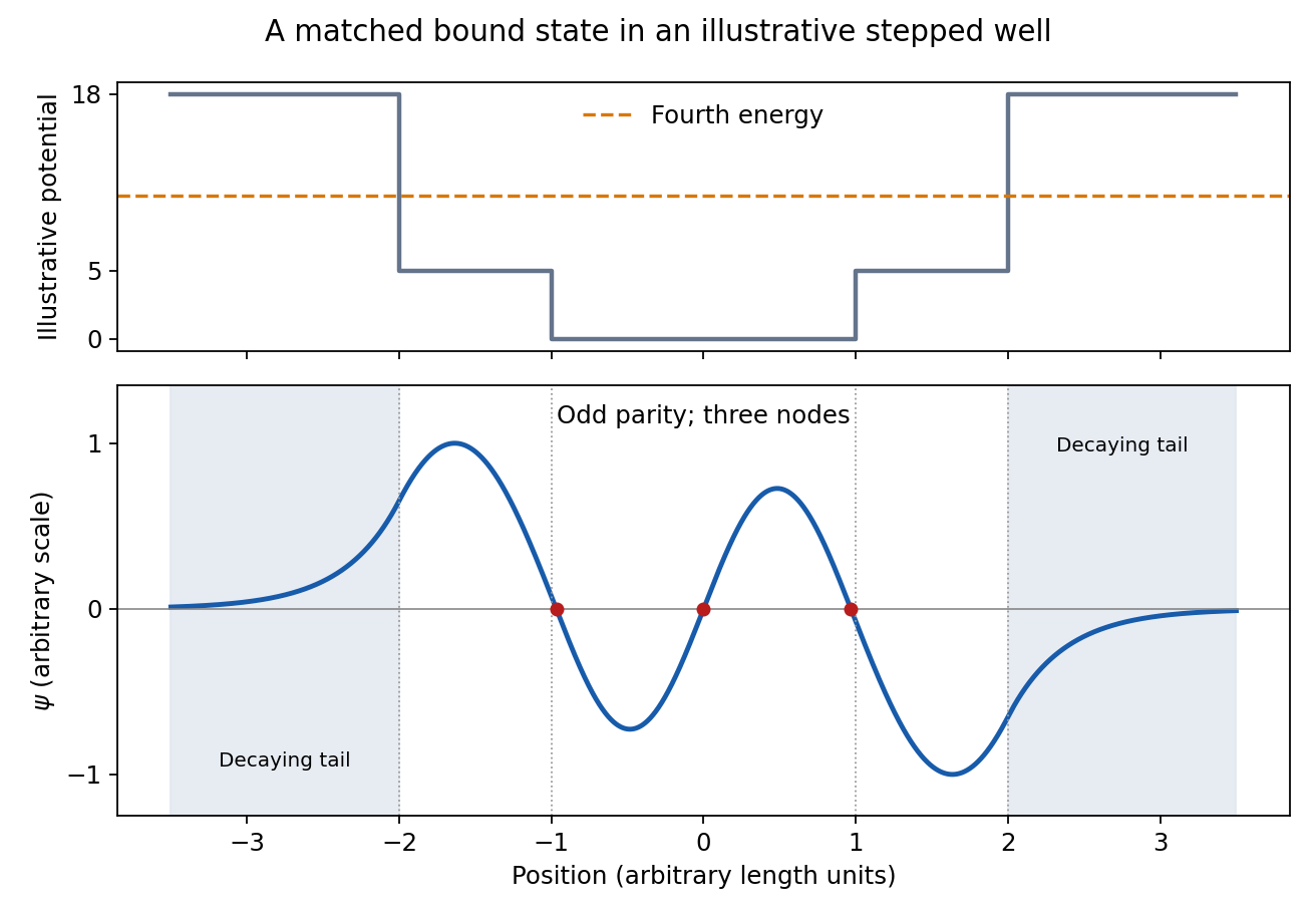
Fourth bound state
. Details. This original wavefunction matching at a finite potential step illustration uses freely chosen well dimensions and energies. It shows the required parity, node count, wavelength ordering and decaying tails; the source drawing supplies no numerical scale from which to fix exact node positions.
Past exam of the physics A course of the University of Cambridge 2011 Paper 2 Section A 1 Solution by Codex 0 2026-10-20
Codex 0 2026-10-20For a normalizable state take . inverse construction of a quantum potential gives . differentiation yields , so the chosen potential energy zero fixes . ThusThis energy lies above the negative minima of the potential energy; its zero value does not mean zero kinetic energy. The nodeless eigenfunction is the ground state.
Pinned article: Introduction to the OurBigBook Project
Welcome to the OurBigBook Project! Our goal is to create the perfect publishing platform for STEM subjects, and get university-level students to write the best free STEM tutorials ever.
Everyone is welcome to create an account and play with the site: ourbigbook.com/go/register. We belive that students themselves can write amazing tutorials, but teachers are welcome too. You can write about anything you want, it doesn't have to be STEM or even educational. Silly test content is very welcome and you won't be penalized in any way. Just keep it legal!
Intro to OurBigBook
. Source. We have two killer features:
- topics: topics group articles by different users with the same title, e.g. here is the topic for the "Fundamental Theorem of Calculus" ourbigbook.com/go/topic/fundamental-theorem-of-calculusArticles of different users are sorted by upvote within each article page. This feature is a bit like:
- a Wikipedia where each user can have their own version of each article
- a Q&A website like Stack Overflow, where multiple people can give their views on a given topic, and the best ones are sorted by upvote. Except you don't need to wait for someone to ask first, and any topic goes, no matter how narrow or broad
This feature makes it possible for readers to find better explanations of any topic created by other writers. And it allows writers to create an explanation in a place that readers might actually find it.
Figure 1. Screenshot of the "Derivative" topic page. View it live at: ourbigbook.com/go/topic/derivativeVideo 2. OurBigBook Web topics demo. Source. - local editing: you can store all your personal knowledge base content locally in a plaintext markup format that can be edited locally and published either:This way you can be sure that even if OurBigBook.com were to go down one day (which we have no plans to do as it is quite cheap to host!), your content will still be perfectly readable as a static site.
- to OurBigBook.com to get awesome multi-user features like topics and likes
- as HTML files to a static website, which you can host yourself for free on many external providers like GitHub Pages, and remain in full control

Figure 2. You can publish local OurBigBook lightweight markup files to either OurBigBook.com or as a static website.
Figure 3. Visual Studio Code extension installation.
Figure 5. . You can also edit articles on the Web editor without installing anything locally. Video 3. Edit locally and publish demo. Source. This shows editing OurBigBook Markup and publishing it using the Visual Studio Code extension. 
- Infinitely deep tables of contents:



All our software is open source and hosted at: github.com/ourbigbook/ourbigbook
Further documentation can be found at: docs.ourbigbook.com
Feel free to reach our to us for any help or suggestions: docs.ourbigbook.com/#contact