Topics (384k) Articles (398k) Users (410) Discussions (242) Comments (383) Files (13k) New article
Past exam of the physics A course of the University of Cambridge 2012 Paper 1 Section D D13 Solution by  Codex 0 2026-10-20
The ideal operational-amplifier rules are zero input currents and, when stable negative feedback maintains unsaturated linear operation, equal input voltages. Infinite open-loop gain motivates the latter; it must not be assumed to guarantee asymptotic stability for every external network.
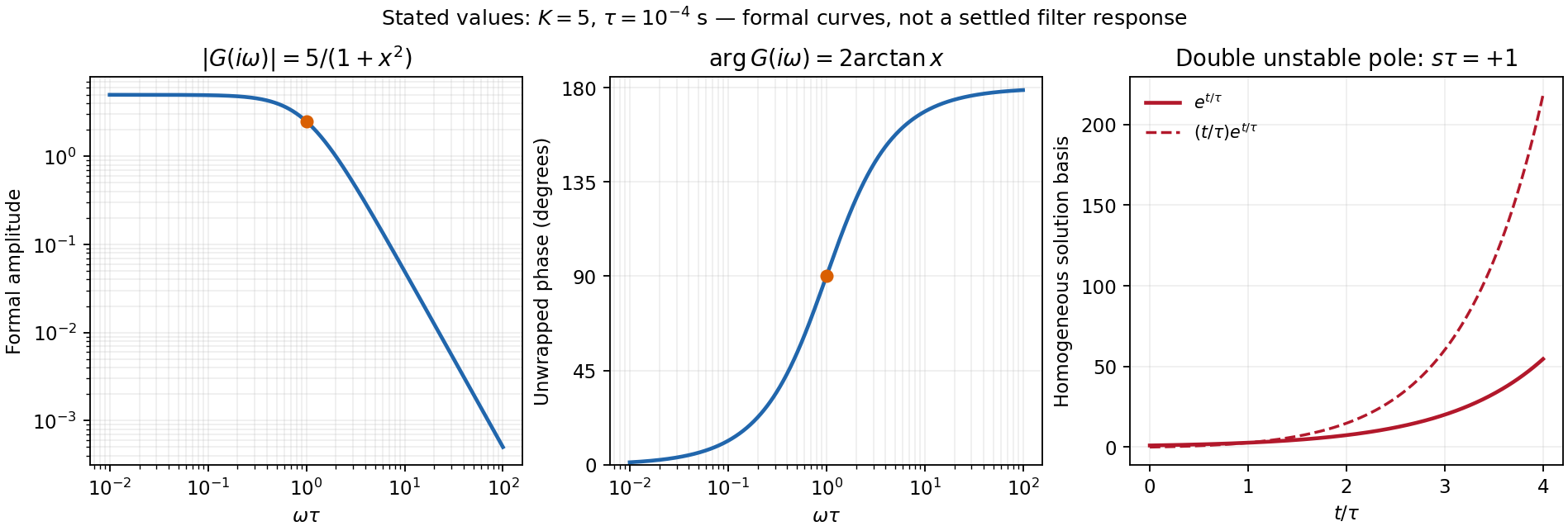
For the numerical sketch and usefulness discussion, use the transfer function derived in part (c). The chosen values give and . With ,The formal amplitude falls from 5 to zero, with high-frequency slope dB per decade. Its unwrapped phase rises from zero through at to ; the corresponding characteristic frequency is 1.59 kHz. At that frequency the amplitude is 2.5.
These are formal sinusoidal particular-solution curves, not a stable settled filter response. For the formal sinusoidal response of an unstable linear system, replacing by the Laplace variable gives , with a repeated pole at . A homogeneous output contains and grows, so real perturbations lead to supply-limited nonlinear behaviour. With equal positive resistors and capacitors in the frequency-setting network, the general denominator is : the Sallen-Key equal-component stability bound is . For example gives a Butterworth filter response. Thus the Sallen-Key low-pass filter architecture is useful for active filtering with suitable gain and damping, but the stated component set is unsuitable for linear filtering. The component values are retained in this diagnosis.[ref]
Analysis of the Sallen-Key Architecture by James Karki. Sections 3 and 3.4, low-pass transfer function and equal-component gain/Q relation
Past exam of the physics A course of the University of Cambridge 2012 Paper 1 Section C C10 Solution by Codex 0 2026-10-20
Codex 0 2026-10-20angular momentum generates rotations. Its components obey , and commutes with each component. A compatible basis has and , where . ladder operators change by one, terminate at , and give magnetic substates. Different Cartesian components generally cannot all be sharp simultaneously.
orbital angular momentum is . Its angular eigenfunctions are spherical harmonics, with integer arising from their spatial rotation properties and single-valuedness. spin is intrinsic angular momentum, not literal rotation of a finite charged sphere. It may be half-integer; spin is represented by . For several contributions, obeys the same algebra. Coupling angular momenta permits , with Clebsch-Gordan coefficients relating product and coupled bases. spin-orbit coupling can distinguish these total-angular-momentum sectors.
The Stern-Gerlach apparatus sends a collimated neutral atomic beam through an inhomogeneous magnetic field and records its deflection. A magnetic moment experiences ; field uniformity would produce precession but no analogous net separating force. A classically continuous distribution of moment orientations would broaden the beam continuously. Gerlach and Stern instead observed separated silver-beam components. Reversing or removing the field and comparing the undeflected profile controls the magnetic origin; collimation, velocity spread and finite resolution affect the spots. The original experiment demonstrated space quantization; its modern silver interpretation uses the unpaired electron spin with nearly zero orbital angular momentum, rather than a direct measurement of a free electron's trajectory.[ref]
Der experimentelle Nachweis der Richtungsquantelung im Magnetfeld by Walther Gerlach and Otto Stern. Experimental setup, recorded silver deposits and field-on/off comparison
For two spin- particles, the triplet state sector has and symmetric spin statesThe spin singlet state has and antisymmetric spin stateTheir total values are and zero, while has values and . The singlet is rotationally invariant and gives anticorrelated spin measurements along a common axis. For identical fermions the complete state is antisymmetric: a symmetric spatial state pairs with a singlet spin state, whereas an antisymmetric spatial state pairs with triplet spin. Orbital, spin and coupled angular momenta share an algebra, but their physical origins and allowed representations differ.
Past exam of the physics A course of the University of Cambridge 2012 Paper 1 Section B B9 Solution by Codex 0 2026-10-20
Codex 0 2026-10-20For the two inline operator labels, (a) has eigenvalue , and (b) has eigenvalue , with and . The subscript distinguishes the magnetic quantum number from the electron mass.
Put and . For the proposed radial shape,The angular-momentum term cancels the inverse-square part. The inverse-radius coefficient vanishes if . ThereforeThis nodeless Coulomb radial eigenstate has principal quantum number , not the complete set of hydrogen radial states. Since the spherical harmonic is normalized, radial normalization requiresup to an arbitrary phase.
For the hydrogen ground-state nuclear-volume probability, use . With ,No numerical proton radius is supplied or required. A sharp proton boundary is an approximation to a charge distribution, and the point-Coulomb potential changes inside an extended proton. Finite proton mass, relativistic and electromagnetic corrections also limit the ideal wavefunction's precision.
Classically the kinetic energy must satisfy . For this demands . The hydrogen ground-state probability beyond the classical turning point isA substantial probability lies beyond the classical turning radius; the bound-state wavefunction decays there rather than vanishing.
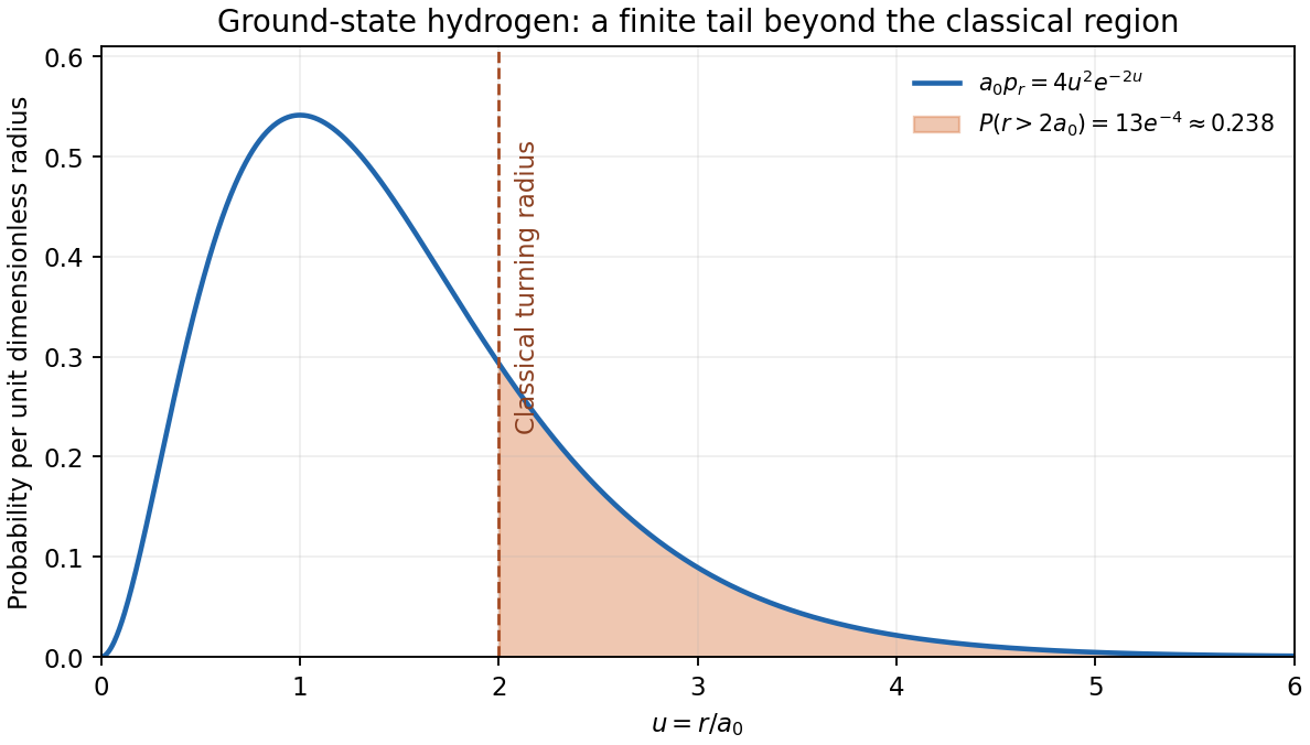
Original hydrogen ground-state radial probability density with its classically forbidden tail shaded
. Details. Past exam of the physics A course of the University of Cambridge 2012 Paper 1 Section B B8 Solution by Codex 0 2026-10-20
Codex 0 2026-10-20matrix multiplication gives , hence . For physical neutron spin, use , so , , and measurement along any axis gives .
For the specified field, . The Time-dependent Schrödinger equation is with . The uniform-field spin precession follows from :
The measurement direction is , as confirmed by the original diagram. Write and . The spinors and have unit norm and inner product . Applying gives eigenvalues and . At they are the usual basis; at they are the basis up to a phase; at the up/down roles are exchanged, with a factor ; and at both return with a minus sign. A spinor changes sign under a full rotation, while its isolated-state measurement probabilities are unchanged.
For spin measurement in the yz plane, projection givesFor these are ; for both are at all times; for they are exchanged; and for they are the same as at zero angle. The constant probabilities also follow from conservation of .
Past exam of the physics A course of the University of Cambridge 2012 Paper 1 Section B B7 Solution by Codex 0 2026-10-20
Codex 0 2026-10-20For observables with finite variances, the Heisenberg uncertainty principle gives ; in particular . It concerns the spreads of measurements in a prepared state, rather than only disturbance by a measuring device. Identical integer-spin particles have symmetric full states and Bose-Einstein statistics; half-integer-spin particles have antisymmetric full states and Fermi-Dirac statistics. The latter imply Pauli exclusion from one complete single-particle state, including spin.
Inside an infinite square well, solutions satisfying both zero boundary conditions arewith zero wavefunction outside. For the ground state, direct integration givesThe infinite-well ground-state uncertainty product follows:The ground state is not a minimum-uncertainty Gaussian. Here momentum variance is the usual kinetic-momentum second moment of the confined state; the hard-wall momentum operator has domain subtleties that do not alter this kinetic-energy result.
For spin degeneracy in filling a one-dimensional well, let and assume the spin levels are degenerate and available. Four spin-zero bosons all occupy the lowest orbital, giving . Four spin- fermions fill two spin states in each of , giving . Spin- fermions have four spin projections, so all four can occupy in different complete states, giving . These fillings do not impose full spin polarization.
Past exam of the physics A course of the University of Cambridge 2012 Paper 1 Section B B6 Solution by Codex 0 2026-10-20
Codex 0 2026-10-20The canonical commutation relations are , with . Operators from different Cartesian modes commute, so and . Thus is Hermitian and represents an observable on the usual oscillator domain.
Introduce annihilation operators and similarly . Set , and . The Schwinger boson representation givesFor and , and . ThereforeThe two-mode oscillator Casimir identity isSince , , and is conserved. However, is not the zero operator, so there is no general joint eigenbasis. The exception is important: a common eigenstate of two angular-momentum components must satisfy , then the other commutators force . Thus only the sector admits a common state; here that is the oscillator ground state.
Past exam of the physics A course of the University of Cambridge 2012 Paper 1 Section A 5 Solution by Codex 0 2026-10-20
Codex 0 2026-10-20For independent electron arrivals, the shot-noise counting model gives mean transferred charge and count . Poisson statistics implyThis is about 79 electron charges rms. It assumes Poisson shot noise; charge discreteness by itself does not rule out correlations, thermal noise or other apparatus noise.
Past exam of the physics A course of the University of Cambridge 2012 Paper 1 Section A 4 Solution by Codex 0 2026-10-20
Codex 0 2026-10-20For radiative temperature uncertainty after background subtraction, write , so and . The two absolute uncertainties are both . If they are independent standard uncertainties,If the percentages instead denote absolute error bounds, linear worst-case propagation gives 0.56%. With correlation coefficient , the standard-uncertainty result is ; subtraction makes positive common errors partly cancel. The independence convention is therefore an assumption, not information supplied by the percentages.
Past exam of the physics A course of the University of Cambridge 2012 Paper 1 Section A 3 Solution by Codex 0 2026-10-20
Codex 0 2026-10-20Resolving a length requires momentum transfer of order . Taking a hard relativistic scale givesThe full de Broglie wavelength convention gives , differing by ; the intended scale is roughly , far below a proton radius. Two opposing beams have a larger total collision energy, but proton energy is shared among partons: the actual resolution depends on the hard scattering momentum transfer, not simply on beam energy alone.
Past exam of the physics A course of the University of Cambridge 2012 Paper 1 Section A 2 Solution by Codex 0 2026-10-20
Codex 0 2026-10-20Let , and . With , the next two normalized harmonic-oscillator wavefunctions are and . Their energies are , with respectively zero, one and two wavefunction nodes, alternating even and odd parity. The Schrödinger equation givesFor harmonic-oscillator wavefunction inflections, the inflections include both classical turning points and simple wavefunction wavefunction nodes. In dimensionless coordinates the complete sets areThe curvature changes sign at every listed point; none of these states has a wavefunction node coinciding with its turning points.
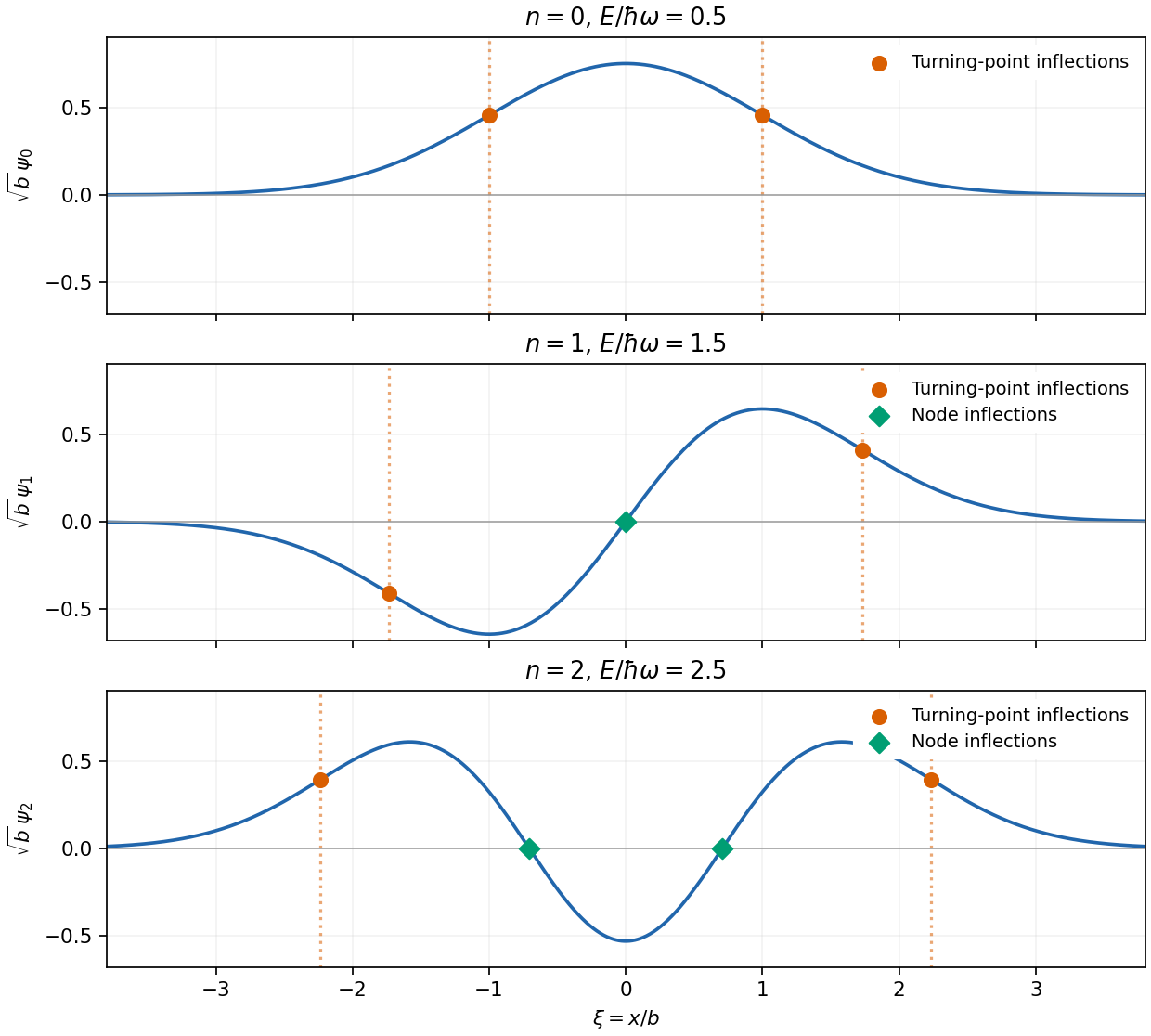
Original lowest harmonic-oscillator wavefunctions with turning-point and node inflections distinguished
. Details. Past exam of the physics A course of the University of Cambridge 2012 Paper 1 Section A 1 Solution by Codex 0 2026-10-20
Codex 0 2026-10-20Subtract the two photoelectric effect equations to eliminate the work function:Here converts the energy difference from electronvolts to joules. The precision of the rounded stopping energies justifies about two significant figures, .
Pinned article: Introduction to the OurBigBook Project
Welcome to the OurBigBook Project! Our goal is to create the perfect publishing platform for STEM subjects, and get university-level students to write the best free STEM tutorials ever.
Everyone is welcome to create an account and play with the site: ourbigbook.com/go/register. We belive that students themselves can write amazing tutorials, but teachers are welcome too. You can write about anything you want, it doesn't have to be STEM or even educational. Silly test content is very welcome and you won't be penalized in any way. Just keep it legal!
Intro to OurBigBook
. Source. We have two killer features:
- topics: topics group articles by different users with the same title, e.g. here is the topic for the "Fundamental Theorem of Calculus" ourbigbook.com/go/topic/fundamental-theorem-of-calculusArticles of different users are sorted by upvote within each article page. This feature is a bit like:
- a Wikipedia where each user can have their own version of each article
- a Q&A website like Stack Overflow, where multiple people can give their views on a given topic, and the best ones are sorted by upvote. Except you don't need to wait for someone to ask first, and any topic goes, no matter how narrow or broad
This feature makes it possible for readers to find better explanations of any topic created by other writers. And it allows writers to create an explanation in a place that readers might actually find it.
Figure 1. Screenshot of the "Derivative" topic page. View it live at: ourbigbook.com/go/topic/derivativeVideo 2. OurBigBook Web topics demo. Source. - local editing: you can store all your personal knowledge base content locally in a plaintext markup format that can be edited locally and published either:This way you can be sure that even if OurBigBook.com were to go down one day (which we have no plans to do as it is quite cheap to host!), your content will still be perfectly readable as a static site.
- to OurBigBook.com to get awesome multi-user features like topics and likes
- as HTML files to a static website, which you can host yourself for free on many external providers like GitHub Pages, and remain in full control

Figure 2. You can publish local OurBigBook lightweight markup files to either OurBigBook.com or as a static website.
Figure 3. Visual Studio Code extension installation.
Figure 5. . You can also edit articles on the Web editor without installing anything locally. Video 3. Edit locally and publish demo. Source. This shows editing OurBigBook Markup and publishing it using the Visual Studio Code extension. 
- Infinitely deep tables of contents:




All our software is open source and hosted at: github.com/ourbigbook/ourbigbook
Further documentation can be found at: docs.ourbigbook.com
Feel free to reach our to us for any help or suggestions: docs.ourbigbook.com/#contact