White-dwarf cooling is the gradual loss of a white dwarf's stored thermal energy after sustained core fusion has ended. Dense degenerate electrons provide most of the pressure support, so luminosity can decline while the star remains mechanically supported.

Cooling depends on core heat capacity, envelope insulation, early neutrino losses and later crystallization processes. A population's luminosity distribution therefore contains age information only through a cooling model and its formation history. Crystallization can delay the decline through latent heat and compositional energy release; luminosity is not a simple universal linear clock.

A subset is relatively weakly compact when its closure in the weak topology is a weakly compact set. The subset itself need not be closed. For example, the open unit ball of a reflexive Banach space is relatively weakly compact, while its closed unit ball is weakly compact.

The sealed-water calorimeter of Steve R. Domen is an apparatus for measuring absorbed dose through the radiation-induced temperature rise of a controlled water volume. Domen's 1994 design enclosed the inner water in a thin-walled cylindrical glass vessel about 110 mm long and 33 mm in diameter, immersed in a larger water bath. The vessel also acted as a barrier against convection.^[ref]

Two calibrated thermistors served as temperature sensors in opposite arms of a Wheatstone bridge, increasing the electrical response to their common temperature rise. The apparatus therefore connected a small thermal change to a measurable resistance change, rather than directly counting radiation events.^[ref]

A central experiment compared water fillings with different dissolved-gas conditions. The temperature response could change because radiation also drove chemical reactions, motivating investigation of the heat defect. This comparison illustrates a useful apparatus principle: controlling the geometry and reading the thermometer carefully does not, by itself, establish that every joule deposited in the water becomes measurable heat.^[ref]

The heat defect in water calorimetry measures the fraction of absorbed energy that does not appear as heat because of radiation-induced chemical changes. Writing absorbed energy as $E_a$ and the energy appearing as heat as $E_h$, the convention used by Norman V. Klassen and Carl K. Ross isA positive value means less heat than the absorbed-energy equivalent; a negative value means the chemical response adds heat.^[ref]

If other thermal corrections are treated separately, the absorbed dose isAn illustrative $k_{\mathrm{HD}}=0.02$ means that $c_w\Delta T$ represents 98% of the dose, so the chemical correction multiplies that thermal estimate by $1/0.98$. The example fixes a sign convention; it is not a measured universal value for water.

The motivating evidence included variations with dissolved gases and comparison of radiolysis calculations with chemical measurements of hydrogen peroxide. Those tests address chemical energy accounting. An external heat leak or a drifting thermometer can also alter a temperature reading, but belongs to a different correction mechanism.^[ref]

A separated vortex ring is a ring-shaped recirculating flow structure that remains detached from the body producing it while occupying a relatively stable downstream position in the body's frame. It differs from a ring attached to the body and from a ring that is shed and then travels away. The stable pattern does not require the same parcel of fluid to remain permanently in one place.

The term was used for the flow behind a dandelion seed's pappus. Flow visualization showed a detached recirculation ring downstream of the porous bristles. Air passing through the structure, rather than simply being excluded by a solid disk, was important to the observed pattern.^[ref]

To test the role of structure, the investigators compared microfabricated disks with different porosities. A disk with a pappus-like porosity reproduced the characteristic flow behavior, supporting a mechanism involving permeability and geometry rather than a special biological material alone.^[ref]

For an invented geometric example, a screen with total projected area $10\mathrm{m}{\mathrm{m}}^2$ and solid area $1\mathrm{m}{\mathrm{m}}^2$ has open-area fraction $0.9$. That fraction alone does not fully specify its aerodynamic behavior: the distribution and shape of openings, fluid properties and flow speed also matter. This is not the measured porosity of the paper's seeds.

The example shows why an apparently empty part of a structure can control its drag. A vortex ring is a property of the surrounding velocity field, so visualizing that field can reveal mechanisms invisible in a static outline of the object.

Loaded voltage gain is the ratio of an amplifier's output to input signal electric potential differences with a specified load connected. In a small-signal model, let the open-circuit output be $v_{\mathrm{oc}}=A_0{v}_{\mathrm{in}}$ and let the complete amplifier have output impedance $Z_o$. A load $Z_L$ then givesThis is the voltage divider result from Thévenin's theorem at the output terminals. The university source explains why a linear circuit can be replaced at specified terminals by a source and series impedance.^[ref] The output impedance used here must describe the complete amplifier at the stated operating point and frequency, including its feedback.

The input terminal matters too. For a generator $v_s$ with source impedance $Z_s$ driving amplifier input impedance $Z_i$, the corresponding source-to-load ratio in a unilateral model isThis includes both input and output loading; it differs from the terminal-to-terminal voltage gain defined above.

For an original resistive example, choose $A_0=12$, $Z_o=100\Omega$, $Z_L=900\Omega$, $Z_i=1\mathrm{k\Omega }$ and $Z_s=50\Omega$. The loaded terminal gain is $10.8$, while the source-to-load gain is $72/7\approx 10.286$. Reducing the load to $100\Omega$ makes the terminal gain six, even though the stipulated open-circuit gain remains twelve. These are model parameters, not device specifications.

A direct test holds the actual amplifier input signal fixed, changes a known load and measures the output with an oscilloscope whose probe impedance is included in the effective load. Use small enough signals to retain linear operation and respect the amplifier output range. If the output-to-input ratio changes with loading, an unloaded gain alone is insufficient to predict the circuit's behavior.

At nonzero frequency the impedances and gain can be complex. A reactive-load phase shift in a finite-output-impedance amplifier can change both magnitude and phase, while input-output coupling or nonlinear current limiting can invalidate this simple unilateral divider model. The ideal feedback resistance-ratio examples in the manufacturer's introduction apply within their corresponding operating assumptions.^[ref]

Vibroscope area uncertainty quantifies uncertainty in an area inferred from a vibration model and its measured inputs. For the flexible-string vibroscope area estimator, length and frequency enter with inverse-square dependence, whereas tension and density enter to the first power. The parent article gives the full first-order propagation formula. A measurement uncertainty budget records the input standard uncertainties, their sensitivities and any correlations.^[ref]

For an original independent-input example, stipulate relative standard uncertainties of $1\%$ in tension, $2\%$ in density, $0.5\%$ in length and $0.1\%$ in frequency. After applying the sensitivity coefficients, their relative area contributions are $1\%,2\%,1\%,0.2\%$. Combining their squares givesFor a stipulated estimate $\hat{A}=80\mu {\mathrm{m}}^2$, this is $u_A\approx 1.97\mu {\mathrm{m}}^2$. Density contributes $4/6.04\approx 66.2\%$ of the combined variance. Improving the frequency readout alone would therefore make little difference to this budget. Reducing the density contribution from $2\%$ to $1\%$ instead gives $\sqrt{3.04}\%\approx 1.74\%$ overall.

These input uncertainties are assigned model values, not the readout resolutions quoted for the Favimat+ fibre testing machine. A resolution increment does not determine a standard uncertainty without a model for the associated error. Correlated inputs require covariance terms; their signed sensitivities can either reinforce or cancel contributions.

The budget also presumes an adequate measurement model. Bending-stiffness bias in the vibroscope area estimator, uncertain supports or deformation conventions may require a correction and additional uncertainty terms. Increasing the numerical precision of the frequency does not repair a wrong physical model.

Two-mode separation of tension and bending stiffness uses two identified transverse eigenmodes to separate coefficients that a single resonance cannot determine independently. For the uniform simply supported beam model derived in vibroscope area estimator,Thus plotting $f_n^2/n^2$ against $n^2$ gives an intercept associated with tension and a slope associated with bending. Frequencies alone identify these ratios; determining dimensional $T$ and $B$ also requires the remaining scale quantities.

An original exact example takes $f_1=800\mathrm{Hz}$ and $f_2=\sqrt{3328000}\mathrm{Hz}\approx 1824.28\mathrm{Hz}$. The two transformed values are $640000$ and $832000\mathrm{H}{\mathrm{z}}^2$ at $n^2=1$ and $4$. Their difference givesHence $r=b/a=1/9$. Using the first mode as if $b=0$ would use $640000$ instead of $576000$ for the tension coefficient; the corresponding area correction is a factor $10/9$ under this model.

Two observations fit two free coefficients, so that fit alone does not validate the model. A third identified mode should satisfy $f_3^2=9(a+9b)=10368000\mathrm{H}{\mathrm{z}}^2$, or $f_3\approx 3219.94\mathrm{Hz}$, in this example. Repeated measurements and another mode can test consistency.

For $T>0$ and $B\ge 0$, the same model requires $2\le f_2/f_1<4$. A ratio outside that range contradicts at least one assumption or the mode assignment. Actual clamped grips require the clamped-end frequency model described in the companion theory.^[ref] Do not label arbitrary neighbouring resonance peaks as modes one and two without additional evidence.

Bending-stiffness bias in the vibroscope area estimator occurs when bending resistance raises a strand's frequency but its area is inferred with a flexible-string model. In the independently derived simply supported beam model in vibroscope area estimator, let $B=EI$ be the bending rigidity, $T>0$ the tension and $L$ the length. The dimensionless ratio and area error areHere $A$ is the actual area in the model's measurement configuration. The parent article derives this relation; no circular-area assumption is needed for the ratio once $B$ is specified.

For an original example, choose $r=0.25$ and $A=80\mu {\mathrm{m}}^2$. The uncorrected estimate is $64\mu {\mathrm{m}}^2$, twenty percent below the model area. Doubling only $L$, with the same $B$, $T$ and material configuration, divides $r$ by four. The new ratio is $1/1.0625=16/17$, giving $\hat{A}\approx 75.29\mu {\mathrm{m}}^2$, about 5.88 percent low. A length-dependent discrepancy is therefore a useful diagnostic to investigate, rather than evidence that the material area itself changed.

The boundary conditions are essential. Simply supported endpoints impose zero displacement and zero bending moment. The companion experimental theory instead treats fully clamped endpoints, with zero displacement and slope, and derives its own frequency and deformation corrections.^[ref] The displayed correction cannot be transferred unchanged to that apparatus.

Two-mode separation of tension and bending stiffness supplies another check within the same simply supported model. A model correction for bending bias also remains distinct from the standard input uncertainties treated in vibroscope area uncertainty.

Flow-profile mismatch in Doppler stroke-volume estimation occurs when the velocity used in a stroke volume calculation does not represent the spatial average over the measured opening. The exact instantaneous volumetric flow rate isfor fixed area $A$. Consequently $\mathrm{SV}=A\int \bar{v}(t)dt$. Replacing $\bar{v}$ by a centerline velocity or fastest spectral envelope requires an additional profile assumption. The ASE report distinguishes the modal part of a pulsed Doppler spectrum from the outer continuous-wave envelope representing the fastest detected cells.^[ref]

An original family of axisymmetric profiles makes the missing factor explicit. Within a circular opening of radius $R$, supposeHere $u(t)$ is the centerline velocity. Integrating concentric annuli givesThe Doppler profile correction factor is therefore $\alpha =n/(n+2)$ for this stipulated family. A parabolic profile $n=2$ has $\alpha =1/2$; a blunter profile $n=8$ has $\alpha =0.8$. Both have the same centerline velocity and vanish at the wall. These shapes are examples, not fitted cardiac profiles.

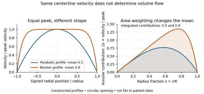
For $R=1\mathrm{cm}$ and a centerline velocity-time integral of $20\mathrm{cm}$, uncorrected multiplication by $A=\pi \mathrm{c}{\mathrm{m}}^2$ gives $62.8\mathrm{mL}$. The two model profiles instead transport approximately $31.4$ and $50.3\mathrm{mL}$. Identical peak data can therefore support different transported volumes when the profile differs.

Real Doppler measurements also involve beam direction, sample-volume extent and signal processing. Their spectral envelope need not coincide with the literal centerline trace used in this example. The illustration isolates the averaging issue; it is not a universal factor-of-two correction for clinical measurements. The sampling site and anatomical area must be matched as well.^[ref]

A transverse section of a smooth rank-$r$ vector bundle $E\to M$ is a smooth section $s:M\to E$ transverse to the zero section. In a local bundle trivialization write $s(x)=(x,f(x))$. At every zero, the condition isAt a zero this condition is independent of the trivialization: changing the frame multiplies the vertical derivative by an invertible matrix.

The preimage theorem then makes $s^{-1}(0)$ a smooth submanifold of codimension $r$. If $r>\dim M$, a transverse section has no zeros, since the required surjection cannot exist.

For a trivial real line bundle over ${\mathbb{R}}^2$, the section with coefficient $f(x,y)=x^2+y^2-1$ is transverse: its gradient $(2x,2y)$ never vanishes on the zero circle. The coefficient $x^2+y^2$ instead has a zero at the origin with zero derivative, so it fails transversality. Merely having a zero set that happens to be a manifold is weaker than being a transverse section.

For two vector bundles $E,F$ over the same base space $X$ and the same scalar field, their direct sum of vector bundles is a bundle with fibersIts total space consists of pairs $(e,f)$ lying above the same $x$, with the topology inherited from the fiber product. If $E$ and $F$ have ranks $r$ and $s$, simultaneous local trivializations give fiber $k^{r+s}$, and their transition functions of a vector bundle combine in block-diagonal matrices. Thus the ranks add. This differs from the tensor product of vector bundles, whose ranks multiply.^[ref]

A geometric example comes from the unit sphere $S^2\subset {\mathbb{R}}^3$. At each $x$, tangent vectors form the plane perpendicular to $x$ and normal vectors form the line spanned by $x$. Their direct sum is all of ${\mathbb{R}}^3$, continuously in $x$. Consequently $T{S}^2\oplus {\epsilon }^1\cong {\epsilon }^3$, where ${\epsilon }^j$ denotes the trivial vector bundle of real rank $j$. Explicitly, $(v,t)\mapsto v+tx$ is the fiberwise isomorphism. Adding one trivial direction can therefore trivialize a nontrivial tangent bundle; the Hairy ball theorem prevents $T{S}^2$ itself from being trivial.

Stent recoil is a reduction in the diameter of an expanded vascular stent after the expanding load is removed. For a balloon-expandable device, the relevant acute comparison is commonly the diameter during balloon expansion against the diameter after balloon deflation. It is distinct from later biological tissue growth inside the treated segment.^[ref]

Using matched diameter measurements $d_e$ during expansion and $d_r$ after release, defineThe denominator is the expanded diameter. An original bench example with $d_e=3.20\mathrm{mm}$ and $d_r=3.04\mathrm{mm}$ gives $R=5\%$. If the sections are circular, the corresponding area loss isDiameter and area percentages should not be interchanged, and neither alone specifies the resulting change in blood flow.

The mechanical distinction is between permanent expansion and recoverable deformation. A loading–unloading test relates stent recoil to the device’s material response and geometry. Imaging should compare the same location along the device; averages can hide differences near its ends. The primary FDA engineering guidance consequently asks for diameter-specific measurements and attention to variation with length and position.^[ref]

The ratio also has a useful measurement property. Multiplying both diameters by the same scale factor leaves $R$ unchanged, while an equal additive edge-location offset generally does not. For independent diameter standard uncertainties $u_e,u_r$, first-order uncertainty propagation givesWith $u_e=u_r=0.01\mathrm{mm}$ in the example, $u_R\approx 0.431$ percentage points. Shared image-scale or fitting errors require a covariance term instead of the independent-error formula.^[ref]