Topics (384k) Articles (398k) Users (410) Discussions (242) Comments (383) Files (13k) New article

For a critical manifold of a fast-slow system , , normal hyperbolicity means that the fast linearization has no eigenvalue with zero real part along the manifold. The slow variables are frozen for this fast subsystem. Uniform estimates on a compact portion require the real parts to remain bounded away from zero.
For , the critical manifold is and the fast derivative is . Its positive- branch is attracting and its negative- branch repelling. At the fold the fast eigenvalue is zero, so normal hyperbolicity fails and the usual fast relaxation can break down.
In the broader dynamical-systems definition, contraction or expansion transverse to an invariant manifold must dominate the tangent dynamics. For a critical manifold of the limiting fast problem, tangent directions are equilibria, giving the stated nonzero-real-part test. A nonzero purely imaginary eigenvalue fails this test even though the Jacobian is invertible.
Two random variables have positive covariance when their centered product has positive expected value:Assume throughout that their second moments are finite. Outcomes where the centered values have the same sign contribute positively; opposite signs contribute negatively. The sign describes their average balance, rather than requiring every outcome to have matching signs.[ref]
Covariance and Correlation by Jeremy Orloff and Jonathan Bloom. §§2–2.1, definition and properties of covariance
A shared group effect can produce positive covariance even when the relation inside each group runs in the opposite direction. For an exact original example, let and be independent random variables with the Rademacher distribution: each takes the values with equal probability. Define and . Both expected values vanish, and independence givesTheir Pearson correlation coefficient is consequently . The four equiprobable outcomes are , , and .
For either fixed value , however, . Thus the conditional covariance is , and the conditional Pearson correlation coefficient is : the two points inside each group lie on a descending line. The law of total covariance identifies exactly where the positive pooled value comes from:The first term averages the conditional covariances; the second measures how the two conditional expectations move together across groups. Here the between-group contribution outweighs the negative within-group contribution. This is a covariance form of Simpson's paradox.
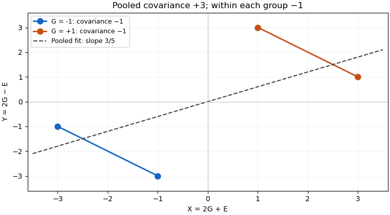
The dashed linear regression line has slope , but that slope does not give the direction of the relation at fixed . Nor does positive covariance by itself establish a causal effect: in the specified model the common variable supplies the positive component. Choosing which variables to condition on is a question about the model and the intended comparison, beyond computing one number.
Positive covariance is also weaker than requiring one variable to be an increasing function of the other. Under appropriate integrability assumptions, strict positive covariance with an increasing payoff supplies a useful sufficient condition; the grouping example shows a different route to the same sign.
Two random variables have negative covariance when , assuming finite second moments. Opposite deviations from their respective expected values then outweigh matching deviations on average. For example, if for a constant , the bilinear identities of covariance give , which is strictly negative when has positive variance.[ref]
Covariance and Correlation by Jeremy Orloff and Jonathan Bloom. §2.1, scaling and covariance with oneself
Sampling without replacement gives a useful example in which the negative sign comes from a shared finite resource. Choose a simple random sample of exactly distinct members from a statistical population of size , with . For each member define the inclusion indicator . Its inclusion probability is . For different members , the joint inclusion probability isSubtracting the product of the expected values givesThe Pearson correlation coefficient follows because each inclusion indicator has variance . Once member is included, only places remain for the other members, reducing member 's conditional probability of inclusion below .
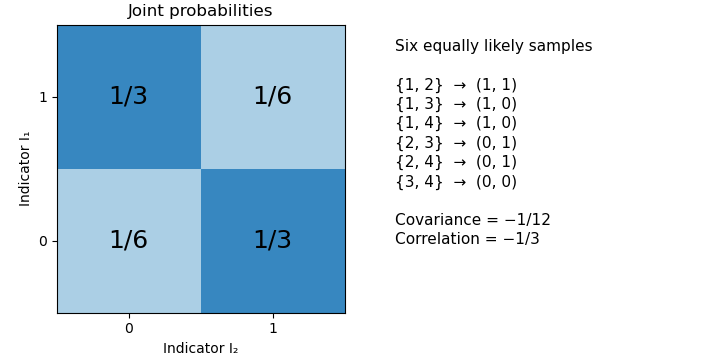
For an original exact example, draw two members from four. The six unordered sample pairs are equiprobable. For , the outcomes and each have probability , while and each have probability . Hence , and their Pearson correlation coefficient is . Matching outcomes remain possible despite the negative covariance.
A fixed total alone does not force every pair among three or more random variables to have negative covariance. If , thenThis constrains the sum of the off-diagonal entries in a row of the covariance matrix. It does not fix each entry's sign. For a counterexample, let be equally likely to be zero or one, and set , , . Their total is always two, yet .
In the simple random sample, exchangeability makes the off-diagonal covariances equal, so the fixed-total identity does determine each of them: . The same distinction between a linear constraint and individual pair signs matters for the joint dependence of leave-one-out consensus residuals.
Spectral common-mode offset rejection is cancellation of an additive frequency-axis shift when the same shift enters two spectral estimates with equal sensitivity and the estimates are subtracted. It improves a frequency difference without establishing accurate absolute frequencies. The relevant measurement model must identify what is shared, and over which observations.
For true frequencies , write measured estimates asThe unknown common offset disappears exactly fromFor independent residual errors of standard uncertainty , the difference still has standard uncertainty . Cancellation of is not cancellation of all measurement noise. With correlated residuals, the covariance term must be retained in uncertainty propagation.[ref]
Evaluation of measurement data — Guide to the expression of uncertainty in measurement by JCGM. Section 5.2, correlated input quantities
An original example uses two spectral positions at and . An additive shift of gives measured positions and , with the same separation. A shared gain error is different: gives separation . Subtraction rejects the offset but retains the scale error.
The algebra generalizes to a contrast of several spectral positions. If and each contains the same additive , its contribution is . Thus weights satisfying reject that offset. Averaging positions with weights summing to one does not. This is an original linear-model derivation of the rejection condition, not a claim that every spectral estimator has this form.
Two failures of the ideal assumption are especially informative. With unequal spectral offset sensitivity, , subtraction leaves . If the offset drifts between observations, it instead leaves . For a stationary drift with variance and correlation at lag , this residual has varianceA common instrument or reference does not alone imply perfect cancellation at different times.
An apparatus-level check measures two stable reference features using the same acquisition and fitting pipeline, then deliberately shifts the assigned axis origin. Their separation should stay fixed under an additive reassignment; a scale change should alter it. Repeated reference observations test temporal drift and residual covariance. In two-dimensional infrared spectroscopy, this test concerns frequency-estimation errors; spectral diffusion also describes physical fluctuations and cannot be identified or removed merely by subtracting an instrumental offset.
A common-origin pressure-tap position error shifts several inferred tap positions together relative to a fixed physical reference. It is a shared contribution to correlated position errors of pressure taps, not an independent placement error for every hole. Whether it affects a pressure-derived load depends on which references are held fixed.
For dimensionless chord coordinate , suppose the uncertain displacement is the same scalar for every tap. A first-order Taylor expansion of the pressure coefficient gives . For a reconstruction with fixed quadrature weights,The position covariance matrix is , a rank-one matrix. Squaring each tap's contribution before adding would discard the shared covariances. The covariance terms belong in the general propagation of uncertainty.[ref]
An original locally linear example takes eight equal weights , equal local slopes and . The reconstructed coefficient has standard uncertainty . Incorrect independence would give . If a two-dimensional load per span is with stipulated dynamic pressure Pa and airfoil chord m, these become and N/m. The chosen slopes describe a sensitivity model, not measured airfoil data.
Opposite-signed sensitivities can cancel the shared contribution. Conversely, repeating coordinate readings without independently checking the misplaced datum cannot average away its fixed error. A proposed test measures an independent reference mark and deliberately translates the assumed origin in the reconstruction, comparing the observed load sensitivity with the derivative above. If moving coordinates also changes the integration weights, those additional derivatives must be included.
Pressure-tap datum cancellation is a different situation. When the tap, leading edge and trailing edge are all expressed through the same affine map , with ,The common origin and scale cancel exactly. Merely translating a shared coordinate system causes no physical tap misregistration. Affine pressure-tap coordinate calibration must therefore state whether the datum is shared or independently fixed before assigning a common-origin uncertainty.
Mass-specific myocardial oxygen delivery expresses oxygen inflow relative to the mass of the represented myocardial tissue. If total coronary oxygen delivery is to mass , the per-mass quantity is . Reporting per givesThe mass and inflow must refer to compatible territories. Normalizing a branch flow by an unrelated whole-heart mass changes the quantity rather than simply changing its units.
An original example has two regions: receiving , and also receiving . Their mass-specific deliveries are and per . The combined value isIt is the mass-weighted mean , not the unweighted mean . Equal total inflows do not imply equal delivery per tissue mass.
Normalization does not remove measurement uncertainty. For small independent input errors,Relative uncertainties in delivery and in mass combine to about . With correlated errors, the relative covariance term must also be included.[ref]
An experimental flow measurement still needs separate oxygen-content and mass information. The primary coronary thermodilution apparatus estimated volumetric flow in a selected artery using infusion and temperature sensing.[ref]
Direct volumetric blood flow measurement in coronary arteries by thermodilution by Wilbert Aarnoudse and others. Abstract, Methods
A mass-normalized oxygen-delivery estimate therefore combines several observations and a territory model.Finally, a regional mean can conceal spatial variation. Two regions can share the same average per-mass delivery while distributing flow differently within them. The denominator makes comparisons explicit; it does not establish uniform perfusion or equal coronary oxygen uptake.
Constraint power transfer is redistribution of energy between parts of a mechanically connected system through constraint forces. An ideal connection may exert nonzero power on each body while exerting zero total power on the combination. Power on a body is the actual force–velocity scalar product; the zero-virtual work property of an ideal mechanical constraint concerns the sum over admissible virtual displacements.[ref]
Advanced Classical Mechanics by Iain W. Stewart. §1.4, equations 1.62 and 1.64–1.66; constrained-system virtual work
An original ideal rigid link calculation makes the cancellation explicit. Let two endpoint positions be and , joined by a massless link of fixed length . SetFor axial tension , the link exerts on A and on B. The powers supplied to the endpoints areThe endpoint velocities need not be identical: the link can rotate. Only their components along the link must agree.
For stipulated and common axial endpoint speed , the link supplies to A and to B. It transfers energy without supplying net energy to their combined system. A load cell measuring axial force and tracked endpoint positions measuring velocities would permit these two powers to be compared. External forces determine how the endpoints subsequently accelerate.
Equal and opposite forces alone do not prove power cancellation. If the connector stretches, and the same axial-force calculation givesAn elastic connector can store the corresponding elastic energy; a dissipative connector can convert mechanical energy into heat. Likewise, an externally prescribed moving support can deliver nonzero net constraint power to a subsystem. The location of the system boundary determines whether a measured exchange is internal transfer or externally supplied work.
The variance of a corrected heterodyne overlap estimate quantifies uncertainty in , where is corrected peak beat current and are separately measured arm currents. The consistency bound for separately measured heterodyne arm powers requires the physical overlap not to exceed one, but measured estimates fluctuate.
For small errors, let have covariance , and put . Linearization givesThus common influences can cancel rather than contribute three independent uncertainty terms. This is the covariance form of the primary measurement-propagation rule.[ref]
For an original model, all three current readings share a multiplicative calibration error, with additional independent errors on each. The common contribution to is zero. The relative standard uncertainty is only , or at overlap . Treating the common calibration error as independent in all three readings would instead give about relative uncertainty.
The common-gain cancellation in heterodyne overlap uncertainty is exact for a single positive gain : replacing by leaves the ratio unchanged. A separate radio-frequency gain uncertainty affecting only does not cancel, nor does an additive dark-current offset generally have this property.
NIST's heterodyne receiver procedure corrected electrical loss and impedance effects separately from matching optical powers and modes.[ref]
Frequency response metrology for high-speed optical receivers by Paul D. Hale and others. PDF pp. 1–2, Heterodyne measurements, equations 1–4
Build the covariance from those actual shared and separate calibration paths. This first-order variance model also needs reconsideration when an arm current is close to zero or background subtraction makes its uncertainty comparable to its value.A samplewise variance upper bound is a nonnegative statistic satisfying , where is the fixed sampling variance at parameter . It controls each realized value outside a probability-zero exceptional set. This implies the expected-value condition for a conservative variance estimator when the expectation exists; the converse fails, as the parent article's counterexample shows. The primary sampling-design definition only asserts the weaker expectation condition.[ref]
Suppose is an unbiased estimator with finite variance, and let . Then Chebyshev's inequality and the samplewise comparison giveNo independence between and the centre is needed. If , unbiasedness makes the centre equal to almost surely, so coverage still holds. This proves confidence bounds from a samplewise variance bound; it does not justify replacing by a normal distribution critical value.
For an original bounded-data example, take independent and identically distributed measurements known to lie in , and estimate their population mean by the sample mean. With , the inequality givesThe deterministic choice is a samplewise variance upper bound for every such population. Thus covers with probability at least . The radius shows the price of distribution-free reasoning; the estimate may be much wider than a model-specific confidence interval.
A conservative variance estimator bounds an expectation, whereas Wald confidence interval coverage is a probability of a joint event involving the centre and its random width. These are different requirements. In the cited sampling-design result, conservativeness means ; the proposition is not a normal-distribution theorem.[ref]
Conservative variance estimation for sampling designs with zero pairwise inclusion probabilities by Peter M. Aronow and Cyrus Samii. §3.1, Proposition 2, expected-value inequality
The rare-large-variance counterexample in conservative variance estimator already shows how little that expectation alone controls coverage.A separate original example isolates the distributional issue even when the variance is known exactly. Let , where is zero with probability and is each of and with probability . Symmetry gives , while . Use the deterministic estimate : it is even a samplewise variance upper bound. Nevertheless,because . Accurate variance alone does not supply the normal distribution of a standardized error. NIST likewise distinguishes multiplying a standard uncertainty by a coverage factor from establishing a confidence level without distributional information.[ref]
Guidelines for Evaluating and Expressing the Uncertainty of NIST Measurement Results by Barry N. Taylor and Chris E. Kuyatt. §§6.2–6.3, conditions for approximately 95 percent expanded uncertainty
The tail assumptions needed for conservative Wald coverage may instead come from an asymptotic normal approximation with a consistent standard-error estimate, or from a justified finite-sample model. If only unbiasedness and a samplewise variance upper bound are available, Chebyshev's inequality gives a different, usually wider, confidence interval. One must establish the centre's bias, the variance condition, and the critical-value argument together.
Detection-threshold selection bias in pulse-energy means occurs when detected pulses have a different energy distribution from all emitted pulses. A detector conditions the reported mean on detection, not merely on emission. Let be emitted-pulse energy with finite mean and let be detection probability conditional on emission . ThenThe denominator must be positive. An ideal energy threshold has above threshold and zero below. Its nondecreasing selection preferentially retains stronger pulses; false triggers or selection on another variable require a different model.
For an original distribution, emitted energies are , and with probabilities , and . Their conditional pulse-energy mean given emission is . A perfect receiver accepting only energies above detects of emitted pulses and reportsThe detected-event mean is about too high for the emitted-pulse mean, even with perfect energy measurements on every accepted event.
A trigger counter, a lower-threshold reference monitor and a threshold sweep can distinguish missing detections from missing emissions. Historical calorimetric inference uses total energy, exposure time and pulse rate; the rate must describe the population whose mean is requested.[ref]
Calibration Service for Laser Power and Energy at 248 nm by Rodney W. Leonhardt. §6.2, Laser Stability, calorimetric pulse-energy inference from energy, injection time and pulse rate
This selection example is an independent probability model, not a reconstruction of that experiment.Known positive detection probabilities can support inverse probability weighting. A hard threshold with zero probability below it leaves that part of the energy distribution unidentified from detected events alone. Reporting the acceptance fraction as well as the detected-event mean makes the conditioning explicit; it does not recover the unseen weak-pulse energies.
A -defined cocharacter of an algebraic torus is a homomorphism of algebraic groupsover . A geometric cocharacter is defined after passing to a separable closure; the cocharacter lattice of an algebraic torus uses these geometric maps with their Galois action. The -defined maps are the Galois-fixed elements.
For , an integer pair gives . Composing with the character yields , defining the integer character-cocharacter pairing. This makes the two geometric lattices dual.
Cocharacters describe algebraic one-parameter subgroups and the integral directions underlying toric cones. For instance, has primitive exponent vector ; Bézout recovers from the coordinates by . The distinction between geometric and ground-field-defined cocharacters matters for nonsplit tori.
Unequal-cluster weighting in a cluster bootstrap must preserve the statistic's intended population target while resampling the independent groups. For group , let be its observed size, its observation sum, and . Two distinct estimates areThe first weights groups by their numbers of observations; the second gives each group equal weight. If group size is related to group response, the corresponding population targets need not agree. For identically distributed independent groups with suitable finite moments, they correspond to and , respectively.
For each cluster bootstrap replicate, draw group slots with replacement and recompute the selected statistic, including its denominator. The Stata manual explicitly notes that unequal group sizes cause replicate row counts to vary; keeping a fixed original row denominator would therefore compute a different statistic.[ref]
Bootstrap sampling and estimation in the Stata documentation. Printed pp. 3–5, Options: size(), cluster(), and idcluster()
For an original two-group example, take and . The original pooled sample mean is , while the equally weighted group-mean estimate is . The four ordered two-group draws have equal probability. Their pooled sample means are , whereas their equally weighted group-mean estimates are .
Consequently the conditional bootstrap expectation of the pooled estimate is , not . This bootstrap ratio bias with unequal cluster sizes is visible with only two observed groups: averaging a random ratio does not generally give the ratio of the averages. It is not a reason to substitute the equally weighted estimate, which changes the estimand, or a claim that every large-group bootstrap is invalid.
Resampling groups in proportion to and then retaining all their rows introduces an additional size preference; that design needs its own justification. Replicated group copies also need distinct identifiers when the fitted model uses those identifiers. The correct resampling unit, the target mean, and the statistic recomputed in each draw must all be specified.
The clipping loss for a triangular pulse is the area removed when a triangular waveform exceeds an amplitude limit. In the ideal model of clipped waveform area, and the upper limit is . The original area is ; the missing top triangle has areaThe geometry is derived in clipped waveform area, with its original diagram. Here is the half-width of the full support, not the width of the clipped plateau.
A useful inverse problem asks how much peak truncation an area-error tolerance permits. If the allowable fractional loss is , the ideal triangle requiresFor an original , pulse, a area-loss allowance requires . At equality, the peak is reduced by but the area changes from to . The plateau duration is only . This is a shape-dependent calculation, not a universal relationship between peak error and integral error.
An attenuated simultaneous trace can test whether the input is approximately triangular and whether its duration stays fixed as amplitude changes. Baseline and bandwidth must be comparable before an area ratio is meaningful. A real saturated integrating amplifier can have additional overload recovery, which the instantaneous clipping model omits.[ref]
ACF2101 Low Noise, Dual Switched Integrator datasheet. p10, Output Overload
The formula supplies a conditional error estimate; it cannot identify an arbitrary missing waveform from its plateau.Adaptive clearance sampling spends more collision detection queries on portions of a trajectory that are difficult to certify, instead of accepting a path merely because a fixed set of samples is clear. Its guarantee comes from a bound on motion between samples. A configuration space path must satisfy the geometric constraints continuously.[ref]
Robotic Systems by Kris Hauser. Chapter 8, Stating the motion planning problem; Chapter 9, clearance
Represent the body by a nonempty compact set and the fixed obstacles by a nonempty closed set. Let be their nonnegative set distance, and suppose a known Lipschitz continuity bound gives . On an interval of duration with endpoint clearances , each time is at most from one endpoint. Hence an endpoint certificate for continuous collision clearance isIf this lower bound is strictly positive, the entire interval is clear. For a required clearance margin , require the bound to exceed instead. Otherwise query the midpoint and subdivide. A sharper certificate uses both endpoint cones; when and the distances satisfy the assumed bound, its minimum is . The simpler bound is sufficient for the example below.
For a translating and rotating rigid body, a valid speed estimate is , where is a bounding radius for rigid-body clearance, provided these are bounds over the whole interval and the obstacles stay fixed. The angular clearance bound for a rotating body proves the rotational contribution. A distance-estimation error bounded by can be accommodated by replacing each reported endpoint distance by its lower bound .
In an original point-motion example, with and passes the obstacle point . Its exact clearance is and suffices. Require . The initial endpoint certificate is positive but below this required margin, so more queries are needed. Recursive midpoint sampling certifies long intervals away from the obstacle and refines only near the closest approach. The stated midpoint rule uses 15 distance queries and certifies 14 intervals. The figure shows the exact function alongside the sampled certificate; the formula is known here only because the example is constructed.
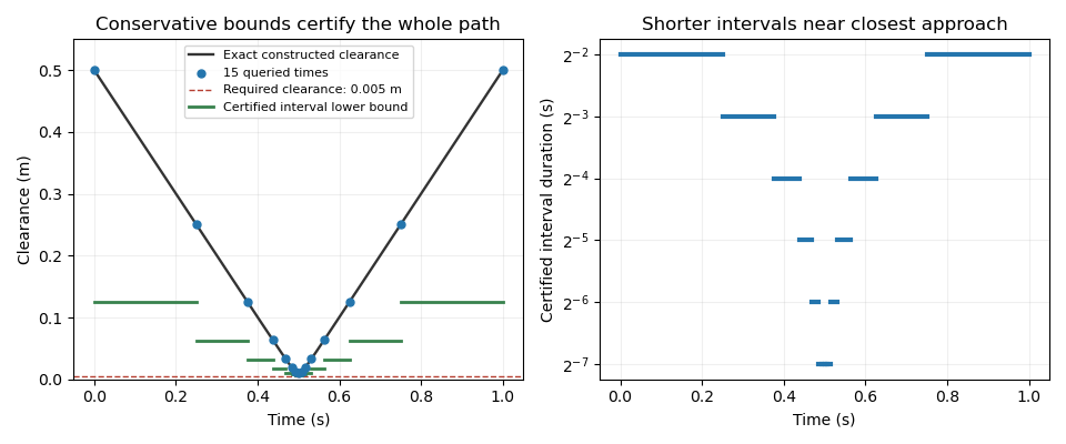
Adaptive endpoint certificates for a trajectory passing 0.01 m from a point obstacle, with a required clearance of 0.005 m. Original exact geometry and recursive midpoint calculation.
Details. Unresolved intervals in adaptive collision checking must remain unresolved if a chosen depth or time budget is exhausted: failure to certify positive clearance does not establish a collision. Conversely, a query with exact zero set distance establishes contact or intersection. A sampled positive distance at or below violates the requested margin but does not establish contact. With exact queries, a valid finite and a trajectory whose clearance has a positive lower bound, subdivision eventually certifies every interval for ; a positive requested margin requires a positive surplus above that margin. Without positive clearance, finite termination is not promised.
A chroma interpolation filter combines retained colour-difference samples to estimate values at the output locations required by chroma upsampling. It acts on the components of YCbCr separately from full-resolution luma. The filter coefficients and the assumed chroma sample location jointly determine the reconstruction. Microsoft's primary conversion guide gives a four-sample interpolation example and states its progressive-scan and edge-handling assumptions.[ref]
For an original one-dimensional linear interpolation rule, let retained samples lie at positions . Define output samples byThe two coefficient sets, one for each output parity, both sum to one. A constant input is therefore reproduced at every output position. With , and , the outputs through are . The values at odd-integer positions are estimates, while the retained even-integer positions are unchanged.
Higher-order interpolation need not remain between neighbouring input values. As an original exact-arithmetic illustration, take a half-position rule with coefficients applied to four consecutive samples. Their sum is one, so constants are preserved. But the sample sequence yields between the two central samples; yields . Negative coefficients permit overshoot. Quantization and clipping then change the result further. The primary Microsoft example uses these interpolation coefficients with integer rounding and clipping.[ref]
Recommended 8-Bit YUV Formats for Video Rendering by Gary Sullivan and Stephen Estrop. four-sample Cout formula and subsequent interpolation discussion
The same numerical coefficients can produce spatially misplaced colour if their assumed input grid is wrong. Centered chroma and co-sited chroma require their actual coordinates to be respected. At image boundaries, missing neighbours require an explicit extension rule. No choice of chroma interpolation filter can uniquely recover arbitrary colour variation discarded by chroma subsampling.
For a circle of radius , a chord with minor central angle has lengthBisecting the isosceles triangle formed by its two radii gives a right triangle with hypotenuse and opposite side , proving the formula.
If the perpendicular distance from the center to the chord is , the same right triangle gives . For , the length is eight. The maximum chord is the diameter , obtained at or .
Chondroitin 4-sulfate is a positional form of chondroitin sulfate with sulfate substitution at the 4-position of N-acetylgalactosamine residues. The modification belongs to a particular position on a sugar residue within the chondroitin chain. It is distinct from changing the chain length or carrying out N-sulfation of glucosamine in a different carbohydrate framework.
Chondroitin 4-sulfotransferase uses PAPS to perform the corresponding positional transfer. The official reaction distinguishes this enzyme from chondroitin 6-sulfotransferase; a shared donor does not imply a shared attachment position.[ref]
An original structural comparison starts with two equal segments, each containing eight complete repeats and sixteen sugar residues. Put one sulfate group at the 4-position of each of the eight eligible amino-sugar residues in the first segment, and instead at the 6-position in the second. Both segments have eight sulfate groups, but their local arrangements differ. Counting groups establishes composition under this model, not the modified position.
This explains why a preparation's name, backbone analysis and positional characterization contribute different information. A proteoglycan containing a chondroitin 4-sulfate chain is also a larger protein–carbohydrate assembly, rather than another name for the isolated sugar chain.[ref]
Pinned article: Introduction to the OurBigBook Project
Welcome to the OurBigBook Project! Our goal is to create the perfect publishing platform for STEM subjects, and get university-level students to write the best free STEM tutorials ever.
Everyone is welcome to create an account and play with the site: ourbigbook.com/go/register. We belive that students themselves can write amazing tutorials, but teachers are welcome too. You can write about anything you want, it doesn't have to be STEM or even educational. Silly test content is very welcome and you won't be penalized in any way. Just keep it legal!
Intro to OurBigBook
. Source. We have two killer features:
- topics: topics group articles by different users with the same title, e.g. here is the topic for the "Fundamental Theorem of Calculus" ourbigbook.com/go/topic/fundamental-theorem-of-calculusArticles of different users are sorted by upvote within each article page. This feature is a bit like:
- a Wikipedia where each user can have their own version of each article
- a Q&A website like Stack Overflow, where multiple people can give their views on a given topic, and the best ones are sorted by upvote. Except you don't need to wait for someone to ask first, and any topic goes, no matter how narrow or broad
This feature makes it possible for readers to find better explanations of any topic created by other writers. And it allows writers to create an explanation in a place that readers might actually find it.
Figure 1. Screenshot of the "Derivative" topic page. View it live at: ourbigbook.com/go/topic/derivativeVideo 2. OurBigBook Web topics demo. Source. - local editing: you can store all your personal knowledge base content locally in a plaintext markup format that can be edited locally and published either:This way you can be sure that even if OurBigBook.com were to go down one day (which we have no plans to do as it is quite cheap to host!), your content will still be perfectly readable as a static site.
- to OurBigBook.com to get awesome multi-user features like topics and likes
- as HTML files to a static website, which you can host yourself for free on many external providers like GitHub Pages, and remain in full control

Figure 2. You can publish local OurBigBook lightweight markup files to either OurBigBook.com or as a static website.
Figure 3. Visual Studio Code extension installation.
Figure 5. . You can also edit articles on the Web editor without installing anything locally. Video 3. Edit locally and publish demo. Source. This shows editing OurBigBook Markup and publishing it using the Visual Studio Code extension. 
- Infinitely deep tables of contents:




All our software is open source and hosted at: github.com/ourbigbook/ourbigbook
Further documentation can be found at: docs.ourbigbook.com
Feel free to reach our to us for any help or suggestions: docs.ourbigbook.com/#contact