Constraint power is the rate of actual work done by constraint forces. For particles with Cartesian velocities ${\mathbf{v}}_i$ and constraint forces ${\mathbf{F}}_i^{\mathrm{c}}$, the total isIt enters the balance of kinetic energy and, after accounting for conservative applied forces, mechanical energy. An ideal mechanical constraint instead imposes zero total virtual work, ${\sum }_i{\mathbf{F}}_i^{\mathrm{c}}\cdot \delta {\mathbf{r}}_i=0$, for allowed virtual displacements at fixed time. Those displacements need not be parallel to actual velocities when the permitted geometry moves.^[ref]

For a smooth ideal restriction $f(\mathbf{r},t)=0$ on one particle, write ${\mathbf{F}}^{\mathrm{c}}=\lambda \nabla f$. Differentiation along its motion gives $\nabla f\cdot \mathbf{v}+{\partial }_{t}f=0$, henceA fixed smooth surface has ${\partial }_{t}f=0$ and zero constraint power. A time-dependent holonomic constraint can have nonzero constraint power even without friction. For example, a bead carried upwards at constant speed $u$ on a horizontal smooth wire receives normal force $mg$ and power $mgu$, increasing its gravitational potential energy. The drive moving the wire supplies that energy.

Zero total constraint power also does not require zero power on every body. Consider two hanging masses connected by a taut, massless, inextensible string over an ideal massless, frictionless pulley. The shared tension is $T$, and the two endpoint speed magnitudes are $v$. If one mass rises while the other falls, the string supplies powers $+Tv$ and $-Tv$: it transfers energy between the bodies while supplying zero net energy to the pair.

With $m_1=0.20\mathrm{kg}$, $m_2=0.30\mathrm{kg}$ and $g=9.81m/{\mathrm{s}}^2$, Newton's second law givesAt $v=0.50m/s$, the two tension powers are $+1.1772\mathrm{W}$ and $-1.1772\mathrm{W}$. Their cancellation leaves gravity's net power, $(m_2-m_1)gv=0.4905\mathrm{W}$, equal to $dK/dt=(m_1+m_2)av$. This constraint power transfer distinguishes an ideal connection that redistributes energy from an externally driven moving support that adds energy to the chosen system.

Coronary thermodilution mixing assumptions are the conditions that make a downstream temperature reading representative of the mixture used to infer coronary blood flow. They include adequate mixing of infused fluid and blood, appropriate volumetric heat capacity values, known infusion rate and temperature, and sufficiently small unmodeled heat transfer between the fluid and surrounding structures.

The apparatus places these assumptions in a concrete setting. In a primary continuous-infusion study, a catheter supplied room-temperature saline while a pressure/temperature guidewire measured distal temperature; the infused-fluid temperature was measured at the catheter tip.^[ref] Temperature at the tip matters because fluid can exchange heat before entering the measured blood flow.

An original two-stream model makes the bookkeeping explicit. Let native blood flow be $Q_b$, infusion rate $Q_i$, baseline blood temperature $T_b$, infused-fluid temperature $T_i$ and mixed temperature $T_m$. Assume equal constant volumetric heat capacity, no external heat transfer and steady complete mixing. Conservation of energy givesand henceNative flow and total downstream mixture flow have different numerators. With constructed $Q_i=20$ mL/min, $T_b=37{}^{\circ }\mathrm{C}$, $T_i=27{}^{\circ }\mathrm{C}$ and $T_m=35{}^{\circ }\mathrm{C}$, the model gives $Q_b=80$ mL/min and $Q_{\mathrm{mix}}=100$ mL/min. This equal-capacity balance is an explanatory model, not the instrument's full calibration algorithm.

Incomplete mixing changes what the sensor observes. If a sensor sampled an unusually cold filament and read $34{}^{\circ }\mathrm{C}$ for the same other inputs, the formula would return about $46.7$ mL/min instead of 80. Repeating that local reading precisely would not correct its lack of representativeness. More generally, a mixed temperature is weighted by transported heat capacity, rather than being an unweighted spatial mean.

Finally, $Q_b$ becomes sensitive to small temperature errors when $T_b-T_m$ is small. At fixed $Q_i,T_b,T_i$,For the constructed example this is $50$ mL/(min K). The derivative describes local sensitivity within the model; it does not estimate errors from incomplete mixing or heat loss. Those require separate physical evidence.

A tensor factor is one of the spaces or modules in a specified tensor product decomposition, such as $V$ or $W$ in $V{\otimes }_{F}W$. The decomposition is part of the data; an abstract vector space need not come with a preferred choice of tensor factors.

For finite-dimensional spaces, $\dim (V\otimes W)=\dim V\dim W$. Thus two two-dimensional factors produce a four-dimensional space, with basis $e_i\otimes f_j$. A vector $v$ from one factor is not itself a tensor-product vector without choosing additional data in the other factor.

A linear operator acting only on the first factor is represented on the product by $A\otimes I_W$, with $(A\otimes I_W)(v\otimes w)=Av\otimes w$. Operators on separate factors commute: $(A\otimes I)(I\otimes B)=A\otimes B=(I\otimes B)(A\otimes I)$. This notation makes independent actions precise, including local operations on composite quantum systems.

For a tensor $T\in V_1\otimes \cdots \otimes V_d$ over a field $k$, its tensor rank is the smallest number of pure tensors needed in an exact expressionThe zero tensor has rank zero. The field and the specified tensor factors are part of the definition. For two factors, the rank agrees with the matrix rank after choosing bases; for three or more factors, one matrix does not capture the full decomposition problem.^[ref]

For instance, $e_1\otimes f_1+e_2\otimes f_2$ has rank two. It cannot be a pure tensor, because its coefficient matrix has two independent columns. Every pure tensor corresponds to an outer-product matrix of rank at most one. In a bilinear algorithm, rank counts the scalar products of linear input expressions needed to form all outputs. Border rank asks the different question of how many terms suffice after allowing a limiting process.

A tensor slice is obtained by contracting one factor of a tensor with a linear functional. For $T\in A\otimes B\otimes C$ and $\alpha \in A^{\ast }$, the contraction $T(\alpha )\in B\otimes C$ is a two-factor tensor and can be displayed as a matrix after choosing bases. Coordinate slices are the contractions with members of a chosen dual basis; their individual matrices depend on that choice.^[ref]

For example, writeThe two first-factor slices are $I_2$ and $N=\left(\begin{array}{cc}0& 1\\ 0& 0\end{array}\right)$. Contracting with $a{e}^0+b{e}^1$ gives the matrix pencil $a{I}_2+bN$, whose determinant is $a^2$. A change of basis in $A$ replaces the generators of this pencil, but does not change its span.

The contraction map $A^{\ast }\to B\otimes C$ is intrinsic. If $T$ is a sum of $r$ pure tensors, its image is contained in the span of $r$ two-factor pure tensors. Its matrix rank therefore gives a lower bound for tensor rank. Studying slices converts a tensor-decomposition problem into restrictions on a space of matrices, although a single slice rank does not generally determine the tensor rank.

Spatial weighting of nail-clipping exposure records determines how much each region of a clipping contributes to a pooled chemical measurement. A concentration reported per unit nail mass is a mass-weighted average. Equal lengths of nail plate need not supply equal amounts of material if width, thickness or density differs.

Let $m(x)$ be mass per unit length at collection and $c(x)$ the retained concentration per unit material mass. For a clipping spanning $[x_1,x_2]$, an original ideal recovery model givesThis assumes complete, composition-independent recovery by the assay. If recovery varies spatially, the measurement equation requires that additional weighting.

For two equal-length regions with masses 1 and 3 mg and stipulated concentrations 0 and 100 units per mg, the pooled concentration is $(1(0)+3(100))/(1+3)=75$ units per mg. A length-weighted average would give 50 and answer a different question. The numerical example illustrates geometry and normalization, not an observed exposure.

Mass-normalized temporal kernels for nail clippings arise when positions are converted into earlier reference-crossing times. If $x=x(s)$ is the material map at collection, the normalized time weighting isAt constant advance speed and uniform line density, the kernel is rectangular, recovering temporal averaging in nail clippings. Variable material geometry or speed changes its shape. A growth experiment following file marks measures displacement over a known interval, not this entire weighting function.^[ref]

A practical study retains segment orientation and measures the material amount used in each assay. Pooling several digits introduces further weights and potentially different growth histories. Wet-mass and structural-mass normalization also differ when water content changes, connecting the issue to hydration versus production in nail mass balance. Specify the denominator and material-to-time map before assigning a pooled concentration to one exposure date.

A speech timing lag is the time difference between corresponding events in two speech recordings. Define ${\Delta }_i=t_{B,i}-t_{A,i}$ for landmark $i$. Positive values mean speaker B's event occurs later; negative values mean B leads. The landmark might be a specified syllable onset or phrase boundary, so its definition is part of the measurement.

In synchronous speech experiments, Fred Cummins recorded paired readings and compared corresponding events. Typical differences were about $40\mathrm{ms}$ on average, with larger mismatches at phrase beginnings.^[ref]

Different summaries answer different questions. For illustrative lags $10,20,-30\mathrm{ms}$, the arithmetic mean is zero, the mean absolute value is $20\mathrm{ms}$, and the root mean square isZero average leadership therefore does not imply close alignment at every event. The square gives larger mismatches more influence on the final statistic.

Recording delays also matter. If channel B adds a known $12\mathrm{ms}$ delay relative to channel A, then ${\Delta }_{\mathrm{recorded}}={\Delta }_{\mathrm{speech}}+12\mathrm{ms}$ under this sign convention. Subtracting that calibrated offset separates equipment delay from speaker timing. Consistent landmark annotation and synchronized recording are consequently necessary for interpreting the measured lag.

Let $p$ be a probability density function on $\mathbb{R}$ with an even function representative satisfying $p(-t)=p(t)$, and suppose $p$ is nonincreasing for $t\ge 0$. For every half-width $a\ge 0$ and center $d\in \mathbb{R}$,Thus a centered interval maximizes captured probability among all intervals of the same width. Symmetry alone is insufficient: mass concentrated in two distant peaks can favor an interval around one peak. The single-central-maximum condition supplied by unimodality is essential.

Here is a direct proof, including densities with jumps. If $F$ is the cumulative distribution function, then $M(d)=F(d+a)-F(d-a)$. Integrability of the density gives absolute continuity of $F$, and hence of $M$ on every bounded interval. Its derivative exists almost everywhere and satisfiesFor $d\ge 0$, one has $|d+a|\ge |d-a|$. Evenness and radial monotonicity therefore give $p(d+a)\le p(d-a)$, so $M^{\prime }(d)\le 0$ almost everywhere. Absolute continuity implies that $M$ is nonincreasing on $[0,\infty )$. Symmetry gives $M(-d)=M(d)$, proving the claim for negative centers too. When $a=0$, all integrals vanish.

An original example uses the triangular distribution density $p(t)=1-|t|$ for $|t|\le 1$ and zero elsewhere. At half-width $a=1/2$,Moving the window a quarter-unit away from the center loses probability even though its length stays1.

The maximizer need not be unique. For a uniform distribution on $[-2,2]$ and $a=1/2$, every center $d\in [-3/2,3/2]$ captures probability1/4. A flat density gives a plateau of equally good intervals. The non-strict form of unimodality, described through interval-shaped superlevel sets, is therefore the appropriate general hypothesis.^[ref]

The lemma applies to a detection time gate when the normalized signal profile is an even unimodal density and the objective is captured signal area. Background noise, asymmetric response or timing uncertainty can change the best gate for another objective; maximizing captured area alone does not optimize every measurement criterion.

A metabolic bilinear form is a nondegenerate symmetric bilinear form $B$ on a finite-dimensional vector space $V$ possessing a vector subspace $L$ withSuch an $L$ is a metabolizer. Equivalently, it is a totally isotropic vector subspace of half the dimension: $B$ vanishes on $L\times L$ and $\dim V=2\dim L$. Nondegeneracy gives $\dim L^{\perp }=\dim V-\dim L$, proving the equivalence.

The symmetric matrix $\left(\begin{array}{cc}0& 1\\ 1& 0\end{array}\right)$ is metabolic: the line spanned by $(1,0)$ is its own bilinear orthogonal complement. Over a field of characteristic different from two, every metabolic symmetric bilinear form is a sum of such hyperbolic planes. In characteristic two, metabolic need not mean alternating: over ${\mathbb{F}}_2$, the identity matrix of size two has metabolizer spanned by $(1,1)$ but has $B((1,0),(1,0))=1$.

Quadrature ambiguity of pressure-tap data means that the same finite set of measured surface pressure values can be consistent with different integrated forces. A chosen quadrature rule fixes an estimate from those readings; it does not, by itself, establish the unsampled distribution. This is an instance of how finite samples do not certify quadrature accuracy.

For an original smooth example, use the normalized airfoil chord coordinate $\xi \in [0,1]$ and let $f=C_{p,l}-C_{p,u}$ be the lower-minus-upper pressure coefficient difference. Put three sample locations at $0$, $1/2$ and $1$, and considerThese polynomials agree at all three taps. Both the composite trapezoidal rule and any other deterministic rule using only these same values produce identical answers for them. Nevertheless,The discrepancy is not caused by a discontinuity or mislocated tap: both profiles are smooth at every sample. At stipulated dynamic pressure $q=400\mathrm{Pa}$ and airfoil chord $c=0.25\mathrm{m}$, the chord-normal pressure loads are $60$ and $70N/m$. Their relation to flow-relative lift still requires the geometric resolution explained in surface pressure integration for airfoil lift.

Additional assumptions can make an error bound possible. If a twice differentiable $f$ has a known bound $|f^{\prime \prime }|\le M$ over the entire chord, the local linear-interpolation remainder gives an integral error at most $M{h}_i^3/12$ on an interval of width $h_i$. Summing givesFor uniform spacing $h$ on this unit interval it becomes $M{h}^2/12$. A value of $M$ inferred only from the same sparse readings is not an independently established bound. Conversely, a justified polynomial model of fixed degree would supply different information and could remove the ambiguity.

A proposed experiment compares the pressure reconstruction with an independently corrected force-balance measurement at matched angle of attack and Reynolds number, then adds taps near suspected sharp features. Pressure-tap position calibration and repeated pressure readings address other error sources. Agreement of two sparse-data rules is a check on their chosen interpolants, not proof that an unresolved contribution is absent.

Spatial resolution of surface-pressure measurements describes which spatial variations of surface pressure can be distinguished by the measurement arrangement. Tap spacing, opening size and the reconstruction model matter separately from uncertainty in each measured pressure. Repeatedly measuring the same taps more precisely does not supply the missing values between them.

A primary wind tunnel experiment by Robert M. Pinkerton sampled a NACA4412 airfoil with 54 pressure orifices and compared measured distributions with theoretical calculations.^[ref] The observations constrain pressures at the instrumented sites. Interpolation and surface pressure integration for airfoil lift require assumptions about the field between those sites.

An original sampling counterexample makes the limitation exact. On a chordwise coordinate $\xi =x/c\in [0,1]$, place five taps at ${\xi }_j=j/4$. Compare two candidate pressure differences,Both give zero at every tap, butAt $A=400\mathrm{Pa}$ and chord $c=0.20\mathrm{m}$, the integrals differ by $40N/m$ in a simplified force-per-span calculation on a flat strip. The geometry and candidate fields are constructed examples, not solutions for a measured airfoil. They prove that these five readings alone do not determine an arbitrary continuous field or its integral.

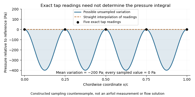
This is spatial aliasing: distinct fields produce the same samples. Additional smoothness or spatial-bandwidth assumptions can constrain reconstruction, but must be stated and tested. The pressure-tap spatial footprint adds another consideration: a finite opening can respond differently from an ideal point measurement. Increasing sampling density, characterizing the probe and checking an independent integrated force address different parts of the inference.

The heliosphere is the region of space dominated by the solar-wind plasma and its carried magnetic field as they interact with the interstellar medium. The solar wind slows at the termination shock and encounters the interstellar plasma at the heliopause.

This is a plasma-interaction boundary, not the outer reach of the Sun's gravity or light. Voyager observations combine particle, magnetic-field and plasma-wave measurements to diagnose the transition. An increased local electron density outside the heliopause supplied an important independent diagnostic, illustrating why a boundary cannot always be identified from one field direction alone.^[ref]

A solar flare is a rapid release of magnetic energy in the solar atmosphere, observed as enhanced radiation and often accompanied by plasma heating and particle acceleration. Emission spans many wavelengths, with different bands tracing different stages and particle populations. A solar flare and a coronal mass ejection can accompany the same eruption, but radiation enhancement and expulsion of magnetized material describe different phenomena.^[ref]

A simple energy scale comes from the magnetic energy density, $B^2/(2{\mu }_0)$. A hypothetical region with $B=0.01\mathrm{T}$ and volume $10^{21}{\mathrm{m}}^3$ containsThis is an illustrative field-energy budget, not a measured flare yield. Only the releasable part of the field energy can power an event; geometry and the final magnetic state matter.

Monitoring depends on the instrument. GOES X-ray sensors measure the Sun's irradiance in specified passbands, including $0.1$–$0.8\mathrm{nm}$. Their time series can locate the rise and peak of an event, while X-ray images locate emitting regions on the solar disc. NOAA's operational event end uses a prescribed fall from peak towards background, so a reported duration is partly a measurement convention.^[ref]

Soft X-rays commonly trace heated plasma, while hard X-ray signatures can track energetic electrons. Comparing their time profiles tests how rapidly released magnetic energy reaches particles and heat. A single bright image or peak flux cannot by itself provide the total energy released in every channel.^[ref]

A stress concentration factor compares a specified local peak stress with a defined nominal reference:It is dimensionless. Both the stress component and the reference geometry belong in its definition; a number quoted without them can be ambiguous. In the infinite circular-hole Kirsch equations, the maximum tangential tension is three times the remote uniaxial stress, so that particular reference gives $K_t=3$.^[ref]

For an original finite-plate normalization example, let width $W=50\mathrm{mm}$, thickness $t=2\mathrm{mm}$, central-hole diameter $d=10\mathrm{mm}$ and tensile force $P=1000\mathrm{N}$. The gross and minimum-net reference stresses areIf the local peak is stipulated as $28\mathrm{MPa}$, the same specimen has $K_{tg}=2.8$ and $K_{tn}=2.24$. In general $K_{tn}=K_{tg}(1-d/W)$ for these reference definitions. This conversion does not solve the finite plate's stress field or predict its peak.

The reference can also be a nominal bending stress or another stress appropriate to the applied loading. A factor obtained for axial tension cannot automatically be reused for a bending problem with different boundary conditions.

An elastic concentration factor is distinct from the crack-tip stress intensity factor, which has units of stress times square root of length. Nor does $K_t$ by itself supply fatigue life or a failure load: yielding, defects, residual stress and the loading history require additional analysis. The factor describes amplification within its stated elastic model.