Chondroitin 6-sulfate is a positional form of chondroitin sulfate characterized by sulfate substitution at the 6-position of N-acetylgalactosamine residues. The numeral identifies a position within a sugar residue; it does not mean that a chain contains exactly six sulfate groups. The alternating chondroitin backbone still contains glucuronic acid and N-acetylgalactosamine-derived residues.

The position can be specified through a defined reaction. Chondroitin 6-sulfotransferase transfers a group from PAPS to the 6-position of eligible N-acetylgalactosamine in chondroitin. Its activity is distinct from that of chondroitin 4-sulfotransferase, which targets a different position.^[ref]

For an original ideal segment, take ten complete two-sugar repeats and suppose every one of its ten eligible amino-sugar residues carries one 6-position substitution. The segment then contains 20 sugar residues and ten sulfate substitutions. Partial modification would change the substitution count without changing the number of backbone residues.

Chondroitin 6-sulfate and chondroitin 4-sulfate can consequently share sugar and sulfate counts while differing in local chemical structure. A total sulfur assay alone cannot identify which positions are modified. Comparing preparations requires stating the structural feature measured, rather than assigning every chain one uniform substitution pattern.^[ref]

A centripetal phase error is a mismatch in the phase of a time-varying centripetal correction relative to the signal being corrected. It is a frequency-specific form of centripetal timing error. A constant centripetal magnitude has no changing phase to misalign, but speed ripple gives an oscillating contribution. For angular velocity $\omega (t)={\omega }_0+\epsilon \cos \Omega t$, expansion of $r\omega (t{)}^2$ to first order in $\epsilon$ gives an oscillation of amplitude $A=2r{\omega }_0\epsilon$ when $r,{\omega }_0,\epsilon$ are positive.

Let the true oscillating correction be $A\cos \theta$ and the applied correction $A\cos (\theta -\varphi )$. Their difference isso its amplitude is $2A|\sin (\varphi /2)|$. Equivalently, phasor subtraction gives magnitude $|A(e^{-i\varphi }-1)|$. Even perfectly matched amplitudes do not guarantee cancellation when their phases differ.

For an original example, $r=0.020\mathrm{m}$, ${\omega }_0=100rad/s$ and $\epsilon =1rad/s$ give $A=4m/{\mathrm{s}}^2$. A phase lag0.10rad leaves amplitude $8\sin (0.05)\approx 0.3998m/{\mathrm{s}}^2$. The centripetal phase-error tolerance for residual amplitude at most $0.10m/{\mathrm{s}}^2$, choosing the small phase-error range around zero, isFor a pure delay $\varphi =\Omega \tau$ at $\Omega =20rad/s$, this corresponds to about1.25ms. The same delay gives a larger phase error at a higher frequency.

A primary rotating-sensor experiment compared internal rotating MEMS sensors with stationary transmission-housing accelerometers; its analysis distinguishes rotating-frame spectral components and reconstruction of a rotation reference.^[ref] The calculation above is an illustrative correction model, not a measured error attributed to that apparatus. A whole-period delay cancels one ideal periodic component, but does not generally align transients or other frequencies.

A Brownian loop soup of intensity $\lambda >0$ in a planar domain $D$ is a Poisson point process of unrooted Brownian motion loops with intensity measure $\lambda {\mu }_D^{\mathrm{loop}}$, where ${\mu }_D^{\mathrm{loop}}$ is Brownian loop measure restricted to loops contained in $D$. Unrooted means that a cyclic change of starting time does not produce a different loop.

For every measurable family $A$ of loops with ${\mu }_D^{\mathrm{loop}}(A)<\infty$, the number of soup loops in $A$ has Poisson distribution with mean $\lambda {\mu }_D^{\mathrm{loop}}(A)$. Counts in disjoint families are independent. Thus the probability that no loop belongs to $A$ is $\exp (-\lambda {\mu }_D^{\mathrm{loop}}(A))$. Finite restrictions give concrete simulation windows even though the whole intensity is infinite.

The conformal invariance of Brownian loop measure, with the appropriate change of time along each loop, gives conformal invariance of Brownian loop soup. Restricting a soup to loops contained in a smaller domain gives the soup there with the same intensity. This couples random loop geometry to conformal restriction measure on simple loops.^[ref]

Uncertainty in a rigid-body bounding radius concerns whether the radius used in a motion bound actually encloses the robot about its declared pivot. A nominal mesh radius can miss manufacturing tolerances, an attached tool or an uncertain reference-point location. The bounding radius for rigid-body clearance must bound the relevant actual occupied geometry, not only a convenient displayed shape.

Let modeled body $\hat{B}$ and modeled pivot $\hat{c}$ satisfy $\Vert \hat{p}-\hat{c}\Vert \le \hat{R}$ for every $\hat{p}\in \hat{B}$. Suppose every point $p$ of the actual body lies within ${ϵ}_B$ of some modeled point, and the actual pivot obeys $\Vert c-\hat{c}\Vert \le {ϵ}_c$. The triangle inequality givesThus a certified radius isThe one-sided geometric coverage assumption is sufficient; it does not require every modeled point to lie close to actual material. A conservative overfilled model is allowed.

For an original example, take $\hat{R}=0.500\mathrm{m}$, shape coverage error ${ϵ}_B=3\mathrm{mm}$ and pivot-location error ${ϵ}_c=2\mathrm{mm}$. Then $R_{\mathrm{cert}}=0.505\mathrm{m}$. A ten-degree rotation about the actual fixed pivot moves any actual point by at mostUsing the nominal radius gives only $87.16\mathrm{mm}$, missing about $0.872\mathrm{mm}$ of possible motion. The angular clearance bound for a rotating body translates that displacement allowance into a clearance bound. Geometry and rotation must be considered together in the continuous-path planning model.^[ref]

Pivot-location uncertainty in a rotational clearance bound is distinct from an uncertain body translation. If the chosen reference point also moves, its translation contributes separately to the occupied-point motion. A speed certificate becomes $v_{\max }+R_{\mathrm{cert}}{\omega }_{\max }$ when the stated translational and angular speed bounds are valid. Substituting a smaller radius about a different center without accounting for that center’s motion changes the problem.

If the geometry has an additional bounded scale factor $s\le 1+{ϵ}_s$ about the modeled pivot, a sufficient bound is $(1+{ϵ}_s)\hat{R}+{ϵ}_B+{ϵ}_c$, under the explicitly separated scale and residual-shape assumptions. With ${ϵ}_s=0.01$ in the example it becomes $0.510\mathrm{m}$. Unknown errors and repeated descriptions of the same geometric tolerance must not be combined as if they were independent extra effects.

A radius enlargement addresses the motion-rate bound. It does not by itself correct an inaccurate sampled distance between the nominal robot surface and an obstacle. That query still needs a suitable geometric allowance or a clearance certificate with bounded distance-query error. Likewise, hard enclosure tolerances are different from standard uncertainties; a root-sum-square of standard deviations is not automatically a guaranteed radius.

A proposed geometric check measures extreme points of the assembled robot, including attachments, relative to the same pivot used by the motion representation. Account for measurement error and verify coverage between sampled surface points using a geometric model or validated tolerance. Recompute the bound when the tool, pivot or assembly changes, and record the radius’s provenance alongside the trajectory certificate.

Finite-shell bias in boundary-density calibration is the difference between a density averaged through a layer of nonzero thickness and the local density at an erosion boundary. Making a layer thinner reduces spatial averaging, but can increase relative uncertainty in the small removed mass and volume. Boundary-density calibration for erosion fronts must manage both effects.

For an original spherical model with outer radius $R$, sampled thickness $\delta$ and smooth radial density $\rho (r)$,Write $s=R-r$. Expanding $\rho (R-s)=\rho (R)-s{\rho }^{\prime }(R)+O(s^2)$ and the volume weight $(R-s{)}^2$ givesThe leading bias is set by the local density gradient. Curvature changes higher-order terms; a uniform density has no such averaging bias, even for a thick shell.

A first-order polymer erosion front speed conversion uses $v=-M^{\prime }/(4\pi R^2{\rho }_s)$, with ${\rho }_s=\rho (R)$. Replacing ${\rho }_s$ by ${\rho }_{\delta }$ givesA density increasing toward the surface therefore leads to overestimated speed when the sampled layer has lower mean density. This calculation assumes a genuine moving front and negligible independent interior density change.

An original local planning model makes the thickness tradeoff explicit. Approximate the sampled area by $A$, the density-gradient magnitude by $|g|$, and the standard uncertainty of removed mass by a thickness-independent $u_M$. Neglect other uncertainties. Squared bias plus variance is approximatelyMinimization givesFor stipulated $A=1\mathrm{c}{\mathrm{m}}^2$, $|g|=0.2\mathrm{g}\mathrm{c}{\mathrm{m}}^{-4}$ and $u_M=0.0001$ g, ${\delta }_{\ast }\approx 0.0316$ cm, or 0.316 mm. At that thickness, bias magnitude and measurement standard deviation are each about $0.00316\mathrm{g}\mathrm{c}{\mathrm{m}}^{-3}$. This is a conditional planning result, not a universal required slice thickness.

Layer-thickness tradeoff in erosion-density sampling also depends on uncertain layer thickness, geometry, conditioning and the accuracy of the gradient model. Shared balance corrections can correlate successive mass differences; the GUM requires those covariance contributions to be included.^[ref]

A proposed check compares several layer thicknesses and looks for a stable extrapolation toward zero thickness, with matched drying and dimensional protocols. A changing gradient or damage caused by sectioning can invalidate the extrapolation. Kureha's polyglycolic acid experiment measures filtered, dried retained solids after water exposure.^[ref] A local shell-density calibration would be an additional measurement, not a quantity already determined by that residue curve.

Photoelasticity is the dependence of a material’s optical response on stress, used to reveal otherwise invisible mechanical patterns. A transparent material that is optically isotropic before loading can become birefringent under load: orthogonal polarizations acquire different refractive indices and therefore a relative phase retardation.^[ref]

For a thin, initially isotropic specimen in a suitable linear regime, the stress-optic law relates induced birefringence to the difference of in-plane principal stresses:Here $C$ is a material coefficient with units $\mathrm{P}{\mathrm{a}}^{-1}$, $t$ is the optical thickness, $\lambda$ the vacuum wavelength and $\delta$ the phase delay. This simple form assumes the relevant stress directions and difference do not change along the light path. A general three-dimensional specimen needs a more careful optical and mechanical model.

With ideal crossed polarizers, intensity normalized to the light after the first polarizer iswhere $\theta$ is the angle between the first polarization direction and a principal optical axis. A dark region can therefore arise from axis alignment or from an integer multiple of $2\pi$ retardation. Darkness alone does not prove that stress is zero.

For illustrative $C=3\times 10^{-12}\mathrm{P}{\mathrm{a}}^{-1}$, $t=5\mathrm{mm}$ and $\lambda =500\mathrm{nm}$, one full phase cycle corresponds toThese chosen values illustrate conversion from optical delay to a stress difference, not a calibration for every plastic. The method does not directly recover a hydrostatic stress shared equally by the two in-plane directions.

A polariscope makes the measurement visible. The Illinois teaching apparatus places a specimen between a polarizer and analyzer, applies load with a manual leadscrew, measures it with a load cell and records the pattern with a camera. Monochromatic illumination and adjustable polarization optics separate information about stress directions and differences.^[ref] Comparing patterns as load changes is a motivating experiment in connecting an optical observable to a mechanical model.

The bearing axial travel margin is the smallest remaining distance between the required axial operating range and either limit of the available bearing axial travel interval. It measures how much extra displacement can be accommodated before the assembly reaches a limit. The physical purpose of the non-locating support is to accommodate relative axial displacement, including thermal changes and accumulated dimensional variation.^[ref]

Let physical limits be $[a,b]$, bearing nominal axial setting be $x_0$, and required changes range from $d_{\min }$ to $d_{\max }$. The two end margins and their worst value areA negative margin means that at least one required position is outside the available interval. Zero means touching a limit, with no reserve in that direction.

For an original example, $[a,b]=[-0.30,0.30]\mathrm{mm}$, changes $[-0.17,0.23]\mathrm{mm}$ and setting $x_0=-0.03\mathrm{mm}$ give $m_{-}=m_{+}=0.10\mathrm{mm}$. A bearing axial setting tolerance of $\eta \in [-0.04,0.04]\mathrm{mm}$ expands the possible operating range to $[-0.24,0.24]\mathrm{mm}$. The guaranteed margin is then0.06mm. Choosing $x_0=0$ would instead give a guaranteed margin of only0.03mm under the same uncertainty bound.

In general, a bounded setting error $|\eta |\le ϵ$ changes the guaranteed margin to $m-ϵ$. This follows by reducing the lower end margin with $\eta =-ϵ$ and the upper end margin with $\eta =+ϵ$. A required reserve $m_{\mathrm{req}}$ therefore needs $m\ge m_{\mathrm{req}}+ϵ$. The example can retain a0.05mm reserve with the centered setting and a0.04mm error bound.

A deterministic tolerance bound and a standard uncertainty are different specifications. Replacing the bound by one standard deviation would not preserve the guarantee without additional distributional assumptions. The margin calculation also concerns geometric travel: it does not by itself establish acceptable contact stress, friction or bearing thermal end-stop load after a limit is reached.

The bearing thermal reaction slope is the local rate of change of a bearing assembly's thermal constraint force with temperature along a specified thermal path. For constant combined axial mechanical compliance $C=C_b+C_s$, relative free-expansion rate $\beta$ and an engaged end stop, the linear model givesIts units are force per temperature, such asN/K. It combines thermal mismatch with elastic restraint; it is not a stiffness measured inN/m. The need to accommodate differential expansion motivates locating/non-locating arrangements in the bearing manufacturer's design guidance.^[ref]

For an original one-stop model with initial relative position ${\delta }_0$, gap $g$, uniform temperature change $\Delta T$ and $\beta >0$,The slope is zero while the gap is open and $\beta /C$ after engagement. At the ideal switching point, the two one-sided slopes differ. The stated slope therefore needs the contact state; it should not be applied throughout the open-gap regime.

Take $\beta =2\mu m/K$ and $C=0.125\mu m/N$. The engaged slope is16N/K. If the bearing end-stop engagement temperature corresponds to a40K increase, increases of60K and70K give forces320N and480N. Conversely, those two force measurements would imply a16N/K slope, and a separately established $\beta$ would imply $C=\beta /(dF/dT)=0.125\mu m/N$. This is a possible bearing thermal stiffness identification measurement, not a reported manufacturer's test.

A bench assessment could measure temperature and axial force at successive equilibrated states after engagement. Measuring both shaft and housing temperatures helps distinguish their actual thermal path from an assumed common temperature. The inferred combined mechanical compliance does not separately identify $C_b$ and $C_s$. Temperature-dependent elasticity, friction, changing contact or temperature gradients can make the observed slope vary, while transient heating can produce a path different from the equilibrated one.

As a local sensitivity coefficient, the engaged slope also propagates a temperature contribution to force standard uncertainty: for a known16N/K slope and $u(T)=0.5\mathrm{K}$, that contribution is8N. Uncertainty in the thermal coefficient, compliance and gap requires its own terms, with covariance included when inputs are correlated.^[ref]

The beam shear angle is the small-angle difference between centreline slope and material-section beam cross-section rotation:With transverse coordinate $z$ and kinematics $u_x=-z\theta (x)$, $u_z=w(x)$, the engineering shear strain is ${\partial }_z{u}_x+{\partial }_x{u}_z=\gamma$. The Euler-Bernoulli beam equation imposes $\gamma =0$; a shear-deformable model permits $w$ and $\theta$ to vary independently. The primary beam account distinguishes these kinematics and relates transverse force to the resulting shear measure.^[ref]

For an original local example, suppose shape measurements give $w_x=0.015$, while section markers give $\theta =0.010$ radians in the same sign convention. Then $\gamma =0.005$, about $0.286$ degrees. Setting the section rotation equal to the observed slope would erase this measured discrepancy by assumption.

In a simple linear shear model, the transverse force resultant is $V=S\gamma$, with effective beam shear rigidity $S=k_{s}GA$. Here $G$ is the shear modulus, $A$ the material area, and $k_s$ a section correction coefficient. Stipulating $G=1.0\mathrm{GPa}$, $A=20\mathrm{m}{\mathrm{m}}^2$ and $k_s=5/6$ gives $S=16667\mathrm{N}$ and $V\approx 83.3\mathrm{N}$. The correction coefficient accounts for using a reduced section model; it is not universally fixed at $5/6$.

A physical test must measure both the centreline shape and section orientation, for example by tracking markers during loading. Shape alone determines $w_x$ but cannot independently determine $\gamma$ without section-rotation information or an additional mechanical model. The comparison also requires compatible spatial resolution and angular measurement calibration.

A balloon compliance fixture correction removes the volume response of tubing, connectors, fluid and other apparatus from a measured balloon volumetric compliance. It is a correction to a defined measurement arrangement. The pressure reference and the state of the apparatus must match between characterization and use.

For a quasistatic experiment in which fixture and balloon experience the same pressure increment, writeA separately characterized fixture supplies $C_f$. A rigid termination can provide one control configuration, but changing tubing or trapped gas between the control and balloon runs changes the correction itself.

For an original example, $C_{\mathrm{meas}}=2.00$ and $C_f=0.50\mu \mathrm{L}\mathrm{kP}{\mathrm{a}}^{-1}$ give $C_b=1.50\mu \mathrm{L}\mathrm{kP}{\mathrm{a}}^{-1}$. Assigning the whole measured response to the balloon would overestimate it by one third relative to the corrected value. Independent standard uncertainties $0.05$ and $0.04\mu \mathrm{L}\mathrm{kP}{\mathrm{a}}^{-1}$ give $u(C_b)=\sqrt{0.05^2+0.04^2}\approx 0.0640\mu \mathrm{L}\mathrm{kP}{\mathrm{a}}^{-1}$. Correlated inputs instead require the term $-2\mathrm{Cov}(C_{\mathrm{meas}},C_f)$ in the variance.^[ref]

Trapped gas explains one nonlinear contribution. For an isothermal gas pocket with $p_{\mathrm{abs}}{V}_g$ constant, its local stored-volume response is $-d{V}_g/dp=V_g/p_{\mathrm{abs}}$. A $20\mu \mathrm{L}$ pocket at $100\mathrm{kPa}$ absolute pressure contributes $0.20\mu \mathrm{L}\mathrm{kP}{\mathrm{a}}^{-1}$. Absolute pressure is required here; substituting gauge pressure into the gas law would be wrong.

A manufacturer's diameter-versus-pressure chart, such as Nipro's Thouzer chart, reports a different observable from injected volume.^[ref] Such a chart does not measure the fixture's stored volume. Comparing a measured volume curve with it requires the balloon geometry and apparatus correction, rather than treating diameter compliance and whole-system volume compliance as identical.

During flow, different parts of the fixture can have different pressures. The simple additive quasistatic model then needs a dynamic extension, consistent with the balloon inflation hydraulic time constant. Loading history and hysteresis must also match before two response curves can be subtracted.

A Jacobian area correction for radiant-exposure maps converts a coordinate-space integral into one over the physical receiving surface. For a one-to-one planar calibration map $\mathbf{x}=f(u,v)$,The Jacobian determinant supplies physical area per coordinate-area increment. This change of variables formula preserves the radiant exposure definition as incident energy per receiving area.^[ref]

For an original two-dimensional example, let $0\le u,v\le 1$ and map $x=au$, $y=bv(1+u)$, with $a=2\mathrm{mm}$ and $b=3\mathrm{mm}$. Then $|\det Df|=ab(1+u)$. Stipulate $H(f(u,v))=H_0(1+u)$ with $H_0=2\mathrm{J}{\mathrm{m}}^{-2}$. The physical receiving area is $3ab/2=9\mathrm{m}{\mathrm{m}}^2$, andIts spatially averaged radiant exposure is $28/9\approx 3.111\mathrm{J}{\mathrm{m}}^{-2}$. Uniformly averaging the exposure values over $u,v$ without the determinant gives only $3\mathrm{J}{\mathrm{m}}^{-2}$.

The correction applies to exposure densities represented in distorted coordinates. If each detector sample already reports energy integrated over its physical patch, summing those calibrated energies requires no second multiplication by patch area. Otherwise the area is counted twice. An optical camera reduction must specify whether its values represent energy, irradiance, exposure or a further processed signal.

The sinotubular junction is the distal boundary of the aortic root, where the bulging aortic sinuses transition to the tubular ascending aorta. It lies above the virtual basal ring; high points of the crown-shaped leaflet attachment reach this region at the aortic valve commissures.^[ref]

Its diameter is consequently a level-specific geometric measurement, distinct from a maximum sinus diameter or a basal aortic annulus diameter. A constructed axial outline could have respective diameters of 24, 32 and 28 mm at the basal, sinus and sinotubular junction levels. Those numbers are stipulated geometry, not normal values or a diagnostic threshold. Even perfect measurement cannot make the three levels interchangeable.

A simple blood flow calculation illustrates the consequence of specifying a level. Consider two circular sections in an ideal unbranched conduit carrying the same incompressible volumetric flow rate $Q$. Their mean axial speeds satisfyFor stipulated diameters of 20 and 30 mm, ${\overline{u}}_2/{\overline{u}}_1=4/9$. Increasing a circular diameter by $50\%$ increases its area by $125\%$, so speed does not scale inversely with diameter alone. The calculation is a continuity example; actual aortic root transport has moving boundaries, branching coronary arteries and nonuniform velocity.

The sinotubular junction also describes part of the supporting geometry of the aortic valve. Distance between commissural attachment sites and the shapes of the valve leaflets are different descriptors from one diameter. Understanding the junction therefore helps relate an anatomical outline to leaflet coaptation, while a single diameter cannot establish the complete closing geometry.

An aortic sinus is one of the bulging spaces of the aortic root behind an aortic valve leaflet. In the usual three-leaflet arrangement, two sinuses give origin to the coronary arteries; the third is noncoronary. The distal sinus boundary is associated with the sinotubular junction.^[ref] A sinus is thus a local part of the root geometry, rather than the whole ascending aorta or the central passage alone.

The geometry has an experimentally testable role in valve motion. B. J. Bellhouse and L. Talbot placed a rigid-walled valve model in a pulsatile water tunnel. Their primary report describes a trapped circulating flow and a downstream stagnation point within each sinus, with much of leaflet closure occurring before net forward flow had ended.^[ref] This is evidence from a controlled physical model, not direct observation of every patient or proof that root walls are rigid.

A local circulation can coexist with net forward transport. For an original accounting example, suppose an ideal central stream carries 80 mL/s downstream, while an adjacent recirculating region carries 10 mL/s across a selected internal surface in each direction. The circulating contributions cancel in the net flux through that surface even though the fluid there is moving. Thus net volumetric flow rate alone does not specify the spatial velocity field near a leaflet.

The same distinction matters for washout. A sinus can contain rapidly moving fluid whose paths mostly recirculate; speed alone does not establish how quickly that fluid is replaced. Replacement depends on exchange with the through-flow and can be investigated using a tracer or modeled pathlines. The aortic sinus therefore connects a visible anatomical shape with questions about leaflet loading, local flow and transport history.

Aortic root measurement-plane dependence is the change in a reported dimension caused by selecting a different anatomical level or imaging direction. Basal, sinus and sinotubular junction measurements describe different structures. Even at a fixed level, an oblique observation need not equal a dimension obtained in a plane perpendicular to the local vessel direction.

The anatomical exposition illustrates separate root measurement levels in an echocardiography view and distinguishes the basal and sinotubular boundaries.^[ref] The three-dimensional crown of leaflet attachments also differs from a single flat ring.^[ref]

An original ideal circular cylinder example isolates obliquity. Let the true perpendicular radius be $R$. A plane whose normal is tilted by angle $\theta$ from the cylinder axis cuts an ellipse with semiaxesThe longest apparent diameter is $2R/\cos \theta$. For a stipulated perpendicular diameter 30 mm and tilt 30 degrees, it is approximately 34.64 mm, 15.5% larger despite unchanged material geometry.

The ellipse's area is $\pi R^2/\cos \theta$. If the longest diameter were instead inserted into a circular-area formula, the estimate would be $\pi R^2/{\cos }^2\theta$, 33.3% above the true perpendicular area at 30 degrees. Measuring the area of the oblique cut and assuming a circular area from its longest diameter introduce different geometric factors.

An actual aortic root is curved, sinus-bearing and time-dependent; it is not a uniform circular cylinder. The example demonstrates one source of measurement dependence rather than providing a universal correction for patient images. Anatomical asymmetry, selected landmarks and phase of the cardiac cycle must also be recorded.

A reproducible comparison therefore identifies the root level, imaging plane, direction of the reported dimension and cardiac phase. Two numbers should not be treated as a growth observation until their measurement definitions are compatible; a change in plane can change a number without an underlying change in root size.

A Valsalva graft is a synthetic vascular graft with an expanded root region intended to reproduce the sinus-bearing geometry of the aortic root, rather than replacing it with one uniform straight tube. Its shape is relevant to the relationship between the aortic valve, aortic sinuses and sinotubular junction. It is a prosthetic conduit, not a biological valve leaflet.

The original 2000 design report described a modified textile conduit with a locally reoriented corrugation pattern. The modified section could expand circumferentially under pressure to create pseudosinuses, while the adjoining tube retained a different direction of adaptability.^[ref] The engineering idea is to control where the conduit can expand, not simply to increase every dimension uniformly.

An original geometric illustration replaces a uniform circular tube of radius 1 cm and length 5 cm by one whose radius is 1.5 cm over a 2 cm segment and remains 1 cm elsewhere. The additional lumen volume isThe uniform model has volume $5\pi \approx 15.71$ mL and the widened model $7.5\pi \approx 23.56$ mL. These simplified dimensions are not device specifications or sizing instructions, and a stepped circular tube is not the complete three-sinus shape.

Geometric similarity also does not establish identical wall mechanics. A native root and a synthetic conduit can have different pressure-volume responses even if their outlines look alike. A meaningful physical comparison would record geometry and changes in volume or diameter under stated loading, together with leaflet motion or flow measurements as appropriate.

The Valsalva design thus illustrates why a root replacement is a coupled geometry-and-material problem. The source establishes the design and its initial observations; those facts should be kept separate from a blanket claim that every graft reproduces all native compliance or valve behavior.

An atomic displacement ellipsoid visualizes the directional positional spread represented by an anisotropic atomic displacement parameter. For a centered three-dimensional normal distribution with positive-definite Cartesian covariance matrix $U$, its probability surfaces have the formThe eigenvectors of $U$ give the principal directions; if its eigenvalues are ${\lambda }_i$, the semiaxis lengths are $\sqrt{c{\lambda }_i}$. The atomic displacement probability level specifies how much modeled probability is enclosed.^[ref]

The squared Mahalanobis distance ${\mathbf{u}}^T{U}^{-1}\mathbf{u}$ has a chi-squared distribution with3 degrees of freedom in this Gaussian model. A50% ellipsoid uses $c\simeq 2.36597$. Taking $c=1$ instead encloses only about19.9%, so a three-dimensional probability ellipsoid cannot be read as a one-dimensional one-standard-deviation interval.

For an original example, $U=\mathrm{diag}(0.01,0.04,0.09){\mathring{\mathrm{A}}}^2$ gives50% semiaxes approximately0.154,0.308 and0.461 angstroms. An isotropic matrix with the same equivalent isotropic atomic displacement parameter, $U_{\mathrm{eq}}=0.14/3{\mathring{\mathrm{A}}}^2$, instead gives a sphere of radius about0.332 angstroms.

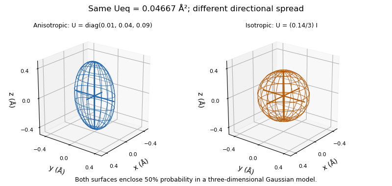
The ellipsoid represents modeled positional spread, including possible static disorder, rather than the atom's physical surface or a confidence region for its refined mean position. Its interpretation depends on the displacement model; the Gaussian probability construction requires a positive-definite covariance and does not turn a negative fitted eigenvalue into a physically meaningful radius.^[ref]

A dipole anisotropy of a radiance field is a directional first-order departure from a constant radiance:Here $\mathbf{\omega }$ is a unit viewing direction, and the bound ensures nonnegative radiance. Writing $\mathbf{b}=ϵ\mathbf{a}$ with unit $\mathbf{a}$ gives the amplitude/direction convention in the title. The angular isotropy test with planar irradiance measurements derives its receiver response.

An original inversion uses opposite receiver orientations. Suppose measured irradiances are $E(+x)=3.4$, $E(-x)=2.6$, and all four $y,z$ readings equal $3.0\mathrm{W}{\mathrm{m}}^{-2}$. The pair means give $\pi L_0=3.0\mathrm{W}{\mathrm{m}}^{-2}$. Sincethe fitted vector is $\mathbf{b}=(0.20,0,0)$. Agreement of the three pair sums is an additional check on this restricted model and a stable measurement chain.

The first angular moment of a radiance field is $\int \mathbf{\omega }Ld\Omega =(4\pi /3)L_0\mathbf{b}$. By contrast, integrating $L$ over all directions gives $4\pi L_0$, independent of $\mathbf{b}$. Thus this example's projected-area-normalized spherical irradiance is $12\mathrm{W}{\mathrm{m}}^{-2}$, exactly the value for an isotropic field with the same $L_0$. One all-direction scalar cannot determine its dipole.^[ref] Receiver angular response must also be characterized rather than assumed ideal.

The amortization gap measures how much evidence lower bound is lost by using the distribution returned by amortized inference instead of the best distribution available for that observation in the same variational family. Hold the generative parameters $\theta$ fixed. Write ${\mathcal{L}}_x(q)$ for the evidence lower bound and suppose the optimum $q_x^{\ast }={\mathrm{argmax}}_{q\in \mathcal{Q}}{\mathcal{L}}_x(q)$ is attained. For the shared rule $q_{\varphi }(\cdot \mid x)\in \mathcal{Q}$,The remaining variational approximation gap is $G_{\mathrm{approx}}(x)=\log p_{\theta }(x)-{\mathcal{L}}_x(q_x^{\ast })$, so the total loss isThus a restrictive recognition network or incomplete training can leave an amortization gap even when the variational family can represent the exact posterior distribution.^[ref]

For an original example, stipulate $p(z\mid x)=N(2x,1)$ for equally weighted observations $x=-1$ and $x=1$. The variational family $\mathcal{Q}=\{N(m,1):m\in \mathbb{R}\}$ represents both posterior distributions exactly when fitted separately, so $G_{\mathrm{approx}}=0$. Restrict the shared rule to $q_b(z\mid x)=N(x+b,1)$: it can adjust the intercept but its slope is fixed at one. The Kullback-Leibler divergence between these unit-variance normal distributions is $(b-x{)}^2/2$. Averaging the amortization gap over the two observations givesThe best shared intercept $b=0$ still loses $1/2$ nat on average. A current rule with $b=1$ loses one nat: half a nat can be removed by training this rule better, while the remaining half requires changing its fixed-slope restriction. This separates the variational family's expressive power from the shared mapping's capacity and current training state.

In a numerical comparison, a locally improved per-observation distribution need not be the global optimum $q_x^{\ast }$. Its improvement supplies a lower bound on the true amortization gap; failing to find an improvement does not establish a zero gap. Comparisons must keep both $\theta$ and $\mathcal{Q}$ fixed.

The alignment padding bound limits the extra bytes needed to move an integer payload address to the next permitted memory alignment. Let $x=a+h$ be the first address after an allocated header, and let alignment require a multiple of a positive integer $A$. Withthe exact bound is $0\le P\le A-1$. It applies to the earliest aligned start, not to arbitrary extra space an allocator may choose to reserve.

To prove the bound, write $k=\lceil x/A\rceil$. The ceiling function gives $k-1<x/A\le k$, hence $0\le Ak-x<A$. Since $P=Ak-x$ is an integer number of bytes, $P\le A-1$. The endpoints can occur: an already aligned $x$ gives zero padding, while $x$ one byte beyond an aligned address gives $A-1$. This is also the statement that $P$ is the least nonnegative residue of $-x$ in modular arithmetic.

For an original example, $A=16$, header size $h=8$ and block start $a=9$ give $x=17$, $p=32$ and $P=15$. The worst-case bound is attained. Starting at $a=8$ instead gives $x=16$ and $P=0$. Identical header and payload sizes can therefore incur different allocation alignment padding at different addresses.

A sufficient address-independent reservation for a payload of $R$ bytes is $h+(A-1)+R$, before any trailer, block rounding or minimum free-block size constraint. For $h=8$, $A=16$ and $R=24$,47 bytes suffice under precisely that layout. A known starting address can require less: $a=3$ needs5 bytes of padding and a37-byte used prefix. Separating the payload from its metadata is the bookkeeping principle illustrated in OSTEP; the bound adds a worst-case alignment allowance.^[ref]

These inequalities concern mathematical integers. An implementation using bounded address arithmetic must separately prevent integer overflow when adding the header, padding allowance or payload. A wrapped sum cannot be justified by a correct bound over unbounded integers.

On the Hilbert space ${\ell }^2({\mathbb{N}}_0)$, the unilateral shift is the bounded linear operatorIt preserves the norm, so $S^{\ast }S=I$. Its adjoint operator shifts the other way: $S^{\ast }(x_0,x_1,\dots )=(x_1,x_2,\dots )$. Consequently $S{S}^{\ast }=I-P_{e_0}$, where $P_{e_0}$ is the orthogonal projection onto the first coordinate.

The range consists of sequences whose first coordinate is zero. Thus $S$ is an isometry but is not onto and is not unitary. Its adjoint has a one-dimensional kernel even though $S$ has zero kernel. These formulas give a concrete infinite-dimensional distinction: in finite dimensions an isometry from a space to itself is automatically onto, whereas the unilateral shift loses one output coordinate.