Topics (384k) Articles (398k) Users (410) Discussions (242) Comments (383) Files (13k) New article

The Kirsch equations describe the stress tensor around a traction-free circular hole in an infinite linear elastic plate under uniform remote tension. For remote stress along , hole radius and polar coordinates measured from that direction, put . In the classical isotropic plane stress model,The fields satisfy equilibrium and the prescribed boundary tractions. They can be obtained using an Airy stress function satisfying the biharmonic compatibility equation.[ref]
Stresses Around a Circular Hole by MIT Materials Science and Engineering. one-page handout, stress function, component equations and boundary conditions
At , , so whileThe tangential stress is at the top and bottom of the hole and at its sides. A traction-free boundary does not require every stress component to vanish: the outward boundary normal is radial, so radial normal and shear tractions must vanish.
For an original distance comparison along , the tangential stress is . At it is , already far below the edge value three. At large distance the polar components approach those of the original uniform Cartesian tension.
A finite-width plate, internal hole pressure, plasticity or out-of-plane bending changes the boundary-value problem. The stress concentration factor three is therefore specific to the stated remote-tension model. The MIT laboratory uses local strain measurements and photoelasticity to examine how actual geometries compare with ideal concentration fields.[ref]
Isotropic Linear Elastic Stress Concentration by MIT Mechanical Engineering. §4.1 and experimental §§6–7
A mini-batch gradient averages gradients of several sampled components of a finite-sum objective. For and batch indices ,With independent uniform draws at fixed , it is an unbiased stochastic gradient: . Its covariance matrix is , where is the covariance of one sampled gradient. The factor follows because centered independent cross terms have expectation zero.
If the indices are sampled uniformly without replacement, the covariance is instead for , when uses the uniform-population normalization. At this gives the exact full gradient. Larger batches reduce sampling variance but require more component evaluations per update; biased sampling or data dependence requires its own analysis.
A mini-batch is a group of training examples processed together in one iteration of a learning algorithm. Its batch size counts examples, while a training epoch usually counts one pass over the available training data. In stochastic gradient descent, a mini-batch gradient combines the component gradients from the selected examples; the group of examples and the resulting numerical estimate are distinct objects.[ref]
Optimizing Model Parameters in the PyTorch tutorials. Hyperparameters and Optimization Loop: batch size, epochs and updates.
For an original counting example, partition eight examples into mini-batches with nominal batch size three and retain the final partial group. The sizes are , giving three updates in one training epoch if each group produces one update. Discarding the final partial group changes which observations participate.
Unequal group sizes also matter when reporting a loss function. At fixed model parameters, suppose the three mini-batch mean losses are . Their unweighted mean is , but the mean over all eight examples isThe smaller last group must not receive the same weight as a larger group when the intended statistic is a per-example sample mean. This bookkeeping issue is separate from the randomness used to select a mini-batch.
SGDR means stochastic gradient descent with warm restarts. Its learning rate schedule repeatedly lowers the learning rate along a cosine curve, then raises it to begin another cycle while retaining the current parameters. Ilya Loshchilov and Frank Hutter's method uses this warm restart to continue an existing optimization trajectory.[ref]
SGDR: Stochastic Gradient Descent with Warm Restarts by Ilya Loshchilov and Frank Hutter. Version5, section3, printed p4
In cycle , let be elapsed training time since the last restart and the cycle duration, measured in the same units. The cosine learning rate schedule isIt starts at , reaches the midpoint of the two bounds at , and reaches at the cycle endpoint. The original implementation updates the elapsed training epoch count within each mini-batch, allowing fractional epoch progress.[ref]
SGDR: Stochastic Gradient Descent with Warm Restarts by Ilya Loshchilov and Frank Hutter. Section3, Eq5 and definition of T_cur
For an original schedule, choose bounds 0 and 0.1, initial duration epochs and duration multiplier 2. The successive cycle lengths are 4, 8 and 16 epochs, with restart boundaries at total elapsed times 4, 12 and 28. In the first continuous cycle, the rates at are respectively .
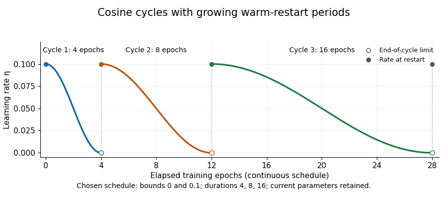
Cosine learning-rate cycles with doubling restart periods
. Own chosen schedule with bounds0 and0.1 and durations4,8,16epochs. Open markers show end-of-cycle limits; filled markers show the rate after restart. The figure plots a schedule, not measured training performance. Details.A discrete convention must specify which update uses the endpoint. For example, sampling phases in the first cycle and restarting before the next step gives rates approximately , followed by . The zero endpoint in the continuous curve is then a limit, rather than an additional zero-rate optimizer step.
Retaining parameters also has a concrete meaning. In an original deterministic gradient descent example with and current , resetting only the schedule leaves . The next step at learning rate0.1 gives0.45; a step at0.01 would give0.495. The restart changes the next movement rather than drawing a new initial parameter. Handling a momentum buffer is a further state convention; restarting the schedule and discarding all optimizer state are different operations. Record cycle phase, durations and rate bounds with an optimization checkpoint.
Clustering groups observations according to a specified notion of similarity or shared structure. Unlike supervised learning, it need not begin with known class labels. The representation, distance and objective determine what counts as a group: nearby numerical values, a connected dense region and membership in a probabilistic component are different criteria.
In K-means clustering, centers minimize the within-group squared-distance objectiveFor fixed groups the minimizing center is their mean; for fixed centers each point is assigned to a nearest center. These elementary minimizations explain the alternating updates. Stuart P. Lloyd's original quantization paper develops the corresponding nearest-representative and mean conditions for scalar signal reconstruction.[ref]
Least Squares Quantization in PCM by Stuart P. Lloyd. Original paper, necessary conditions for least-squares quantizers and iterative construction
For an independent one-dimensional example, the data can be grouped as and , with means and objective . A single center at gives objective . Reducing this objective by allowing more groups does not itself tell us the scientifically appropriate : with one center per observation it becomes zero.
Clustering describes the chosen representation, not an automatic discovery of natural kinds. Changing units can change distances; elongated or nested groups can challenge a squared-distance criterion; different initial centers can produce different fitted solutions. Stability, the scientific question and knowledge of how observations were collected help determine whether a partition is informative.
A training epoch is conventionally one pass through the training data used by an iterative learning procedure. Several parameter updates can occur within that pass. A mini-batch supplies a group of examples for an update, while the epoch counts progress through the data collection rather than counting individual updates.[ref]
Optimizing Model Parameters in the PyTorch tutorials. Hyperparameters, number of epochs and batch size; Optimization Loop, outer epoch and training loop
Suppose there are training examples. Visit each exactly once per pass, form mini-batches of at most examples and retain the smaller final group. Their sizes are . With one update for every mini-batch, an epoch hasupdates. Five epochs therefore make fifteen updates and fifty example visits. Fifty visits do not mean fifty distinct examples: the same ten examples are reused.
Changing the mini-batch size changes the update count. Taking all ten examples together gives one update per epoch under the same rule, while groups of two give five. An epoch count alone consequently does not specify the number of stochastic gradient descent steps, the amount of computation or the final fitted model.
The finite-pass assumption matters. Dropping an incomplete final group in this example gives two updates and only eight visits during that iterator traversal. Reordering the examples on later passes can change which examples are omitted. Sampling with replacement can repeat some examples before visiting others, so a chosen number of sampled updates need not be a literal once-per-example pass. Report those conventions rather than assuming that every loop named epoch guarantees full coverage.
The learning rate schedule needs a declared clock too: changing the learning rate once per epoch differs from changing it once per mini-batch. The optimization tutorial separates the outer loop from the operations that clear gradients, perform backpropagation and update parameters inside the training loop.[ref]
Optimizing Model Parameters in the PyTorch tutorials. Optimizer, zero_grad/backward/step; Full Implementation, nested training and epoch loops
Keeping data passes and update steps distinct makes training runs easier to compare.A directional tipping margin is the distance an interior projection of the center of mass can move along one specified direction before reaching a boundary of its support polygon. It differs from the nearest-edge static tipping margin, which protects against movement in every horizontal direction. For a bounded polygon , interior point , and unit direction , the ray stays inside exactly while all edge inequalities hold. HenceEdges with nonpositive denominator do not limit positive motion along that ray. The underlying gravity-only feasibility criterion is the nonnegative-reaction convex-hull condition in support polygon.[ref]
Robotic Systems by Kris Hauser. Chapter 12, Equilibrium conditions
For an original triangular footprint, take , , in metres and . Moving right gives ; moving downward gives ; moving along gives . The all-direction margin is only , set by the left edge. A displacement allowance restricted to the right can therefore be larger than the isotropic allowance without contradiction.
The same geometry can enter a planar load calculation. A horizontal force applied at height shifts the effective support-resultant point by under the corresponding static torque balance. The directional threshold is , subject also to friction and the other contact assumptions. With and , the rightward example gives , whereas the nearest-edge worst-direction value is .
The scalaron is the additional propagating scalar degree of freedom in a generic nonlinear metric theory of gravity. In the model , it can be expressed in the Einstein frame as a canonically normalized scalar , where is the reduced Planck mass and .
The potential is . Near its minimum, expanding the exponential gives , identifying as the scalaron's small-oscillation mass. At large positive field values the potential flattens, providing the slow-roll mechanism of Starobinsky inflation.[ref]
Embedding (R+R^2)-Inflation into Supergravity by Sergei V. Ketov and Alexei A. Starobinsky. Section I and the pure R-squared contribution to equation (26); scalar potential in the declared Einstein-frame convention
Identifying flow-sensor gain and offset with timed transfers uses a known gas volume delivered over different durations to distinguish multiplicative response from accumulated zero error. In the model , a transfer of volume lasting producesThe observations form a linear regression with design matrix rows . If , gain and offset are identifiable only when the durations are not all equal. Repeating one duration measures the same combination of and more precisely, without separating them.
For two noise-free transfers,Stipulated 3 L transfers lasting 1 and 6 s, measured as 3.020 and 3.120 L, give and . The different durations expose an offset that one transfer could misinterpret as a gain error.
Timing spread and gain-offset estimator covariance quantifies the design. Suppose observations have independent equal volume-error variance , and define . Ordinary least squares givesUnder the stipulated model, wider timing separation improves offset precision. For the two durations above and L, the offset's standard uncertainty is about and the gain's about 0.00406.
The reference syringe volume was treated as known in those formulas. If it is uncertain, repeated sensor tests share that reference uncertainty. Indeed the observations identify only the product when both factors are unknown. Additional repetitions cannot establish an absolute gain without an independently characterized volume. The GUM treats fit uncertainties and common-reference correlations as distinct contributions.[ref]
Guide to the expression of uncertainty in measurement by JCGM. §4.2.5, fitted parameters; §5.2.4, common reference data
The primary spirometry statement's multiple-flow syringe checks test the practical response over different delivery rates.[ref]
Standardization of Spirometry 2019 Update by Brian L. Graham and others. Calibration and Quality Control, 3-L syringe over multiple flows
Actual leaks, flow-dependent nonlinearities and uncertain timing require a richer model than a constant gain and offset.Inverse spectral theory reconstructs an operator or its coefficients from spectral data such as eigenvalues, spectral weights or boundary responses. It asks what the data determine and what additional information is needed for uniqueness.
Eigenvalues alone generally lose information. The matrices and have the same eigenvalues but different entries in the fixed coordinate system. Orthogonal conjugation changes eigenvectors while preserving the spectrum. An inverse problem must therefore specify whether recovery is sought in fixed coordinates, up to a change of basis, or within a more restricted class. Spectral weights can retain information about how selected measurements couple to eigenvectors.
Area weighting of radiant exposure combines patch-average exposures in proportion to the receiving areas they represent. For disjoint patches with areas and mean radiant exposures , the coefficients satisfy , and the combined spatially averaged radiant exposure is . This follows by adding the received energies , rather than averaging a list of values without its geometry.[ref]
An original coordinate example explains a calibration issue in image-based measurements. Let a rectangular receiving strip have length and constant width. Stipulate for . Suppose a calibrated image coordinate maps to physical position . Uniform sampling in is therefore nonuniform in physical area.
The physical area average isAn unweighted average over increasingly dense, uniformly spaced samples would instead converge to . The factor is the change of variables formula's area correction for the chosen mapping; the constant strip width and cancel in the normalized average.
Thus a Jacobian area correction for radiant-exposure maps can matter even if every local exposure value is correct. An optical camera measurement needs its spatial calibration and the receiving-surface map, not just pixel values. Overlapping patches must not be counted as disjoint areas, and local point samples need an explicit quadrature model before they can stand for patch averages.
A box averaging filter gives equal weight to all positions within a specified window and zero weight outside it. In one spatial dimension, its normalized kernel and action areThis is a spatial averaging filter expressed as a convolution. In several dimensions, averaging over an axis-aligned rectangular box uses the product of the one-dimensional kernels.
The discrete counterpart averages a fixed number of samples. On an infinite sequence that is zero except for value ten at index zero, a centred five-sample box average produces value two at indices and zero elsewhere. The total remains ten, while the isolated peak spreads. On a finite array, boundary extension must be specified; reflection, zero padding and wrapping can give different edge values.[ref]
uniform_filter1d in the SciPy documentation. Parameters size, mode and origin: window length, boundary extension and centring
Applying the same box average twice is not the same operation as applying it once. The new kernel is the convolution of the two kernels:Indeed, the integral counts the length of overlap of two intervals, divided by . The resulting support has width , and the weight decreases away from its centre.
For a Fourier mode , one application multiplies the amplitude by ; two applications square this multiplier. The sinc function response explains why a box average smooths a signal without implementing an ideal sharp frequency cutoff. In large eddy simulation, that distinction matters when relating a grid filter to a coarser test filter.
A grid filter defines the resolved field associated with a large eddy simulation, commonly written . Its name reflects the connection between resolved scales and a computational grid, but the filtering operator and the mesh are different specifications. An explicit spatial averaging filter states its kernel; in other methods the retained representation and numerical operations supply an implicit scale selection.[ref]
A dynamic subgrid-scale eddy viscosity model by Massimo Germano and others (1990). §2, original filtered field and coarser test-filter construction
A characteristic width is often related to cell dimensions. One possible three-dimensional convention isCells with widths , and then have . This single number preserves the volume scale but does not describe the strong directional differences of the cell. The filter shape and directional resolution still matter.
Sampling alone also cannot determine which unresolved oscillations were present. At eight equally spaced points on a periodic interval of length , the modes with indices ten and two have identical sine samples:This is aliasing. Removing the high mode by a specified filter before sampling and merely sampling the unfiltered field are different operations.
The subgrid-scale stress depends on the filter actually adopted. A test filter then applies an additional operation to the already resolved data. Reporting only a grid spacing, without the filtering and discretization choices, can leave the mathematical meaning of the resolved field and its closure ambiguous.
The inhomogeneous norm on a domain iswhere the derivatives are weak derivatives. It measures both the size of the function and its first-order variation. The underlying Sobolev space consists of the functions whose first weak derivatives also lie in .
For on , the squared norm is , so the norm is . A nonzero constant has zero derivative but positive norm. Thus the gradient alone defines a seminorm on the full space, not the displayed norm.
On a suitable zero-boundary space over a bounded domain, a Poincaré inequality controls the term by the gradient and makes the gradient norm equivalent to the full norm. The boundary or normalization condition is essential for this replacement.
In finite-population sampling, a simple random sample of fixed size without replacement is a subset of labelled units drawn so that every size- subset has probabilityThe sample is the selected subset; simple random sampling is the procedure that generates it. This definition does not require the observed values to be distinct, only the selected population labels. The without-replacement convention is important because an independent repeated draw from a population is a different design.[ref]
Unequal Probability Sampling in Penn State STAT 506. Lesson 3, simple-random-sampling specialization
One construction randomly orders all labels and takes the first . Each particular subset can occupy those positions in permutations, out of , proving the probability above. Equivalently, draw successively and uniformly from the remaining labels, then discard their order.
For , there are possible samples. A particular unit belongs to four of them, so its inclusion probability is ; a particular pair is one complete sample, so its joint inclusion probability is . These are properties of the procedure before observing which subset was obtained.
A simple random sample need not resemble the whole population in every realization. For fixed values , six of the ten size-two samples contain only zeros. Thus the sample mean is zero with probability , although its expected value is the finite population mean . The remaining four samples each have mean , giving . Unbiasedness concerns repeated selection, rather than a guarantee about any one sample. Coverage of the population labels and faithful implementation of the selection rule remain essential.
Pinned article: Introduction to the OurBigBook Project
Welcome to the OurBigBook Project! Our goal is to create the perfect publishing platform for STEM subjects, and get university-level students to write the best free STEM tutorials ever.
Everyone is welcome to create an account and play with the site: ourbigbook.com/go/register. We belive that students themselves can write amazing tutorials, but teachers are welcome too. You can write about anything you want, it doesn't have to be STEM or even educational. Silly test content is very welcome and you won't be penalized in any way. Just keep it legal!
Intro to OurBigBook
. Source. We have two killer features:
- topics: topics group articles by different users with the same title, e.g. here is the topic for the "Fundamental Theorem of Calculus" ourbigbook.com/go/topic/fundamental-theorem-of-calculusArticles of different users are sorted by upvote within each article page. This feature is a bit like:
- a Wikipedia where each user can have their own version of each article
- a Q&A website like Stack Overflow, where multiple people can give their views on a given topic, and the best ones are sorted by upvote. Except you don't need to wait for someone to ask first, and any topic goes, no matter how narrow or broad
This feature makes it possible for readers to find better explanations of any topic created by other writers. And it allows writers to create an explanation in a place that readers might actually find it.
Figure 1. Screenshot of the "Derivative" topic page. View it live at: ourbigbook.com/go/topic/derivativeVideo 2. OurBigBook Web topics demo. Source. - local editing: you can store all your personal knowledge base content locally in a plaintext markup format that can be edited locally and published either:This way you can be sure that even if OurBigBook.com were to go down one day (which we have no plans to do as it is quite cheap to host!), your content will still be perfectly readable as a static site.
- to OurBigBook.com to get awesome multi-user features like topics and likes
- as HTML files to a static website, which you can host yourself for free on many external providers like GitHub Pages, and remain in full control

Figure 2. You can publish local OurBigBook lightweight markup files to either OurBigBook.com or as a static website.
Figure 3. Visual Studio Code extension installation.
Figure 5. . You can also edit articles on the Web editor without installing anything locally. Video 3. Edit locally and publish demo. Source. This shows editing OurBigBook Markup and publishing it using the Visual Studio Code extension. 
- Infinitely deep tables of contents:



All our software is open source and hosted at: github.com/ourbigbook/ourbigbook
Further documentation can be found at: docs.ourbigbook.com
Feel free to reach our to us for any help or suggestions: docs.ourbigbook.com/#contact