Diameter compliance of a vascular graft quantifies how the measured diameter of a vascular graft changes with distending pressure. A fractional differential convention isThis logarithmic diameter compliance has inverse-pressure units. State whether $D$ is an internal or external diameter and use the same convention throughout a comparison. The distending pressure is lumen pressure minus surrounding pressure.

An interval estimate often uses the lower-pressure diameter as reference:For constructed external diameters $D(80\mathrm{mmHg})=4.00\mathrm{mm}$ and $D(120\mathrm{mmHg})=4.16\mathrm{mm}$, this gives $0.0010\mathrm{mmH}{\mathrm{g}}^{-1}$. Expressed as percent diameter change per 100 millimeters of mercury, its numerical value is $10^4{\overline{C}}_D=10$. The factor $10^4$ combines percent conversion and the 100-millimeter pressure interval; it is not a change in the measured deformation.

A logarithmic interval average instead givesIt differs slightly because its normalization follows the changing diameter. Neither interval value is automatically the local derivative at every pressure.

A primary apparatus measured external vessel-edge motion with video and paired it with transducer measurements of static or pulsatile pressure. The published compliance equation uses systolic and diastolic diameters and pressures, expressed as percent per 100 millimeters of mercury.^[ref] Thus loading frequency, pressure interval and the chosen diameter observable belong to the reported result.

This fractional diameter response differs from volume-based vascular compliance $dV/dp$. For a cylindrical segment with fixed length, $V=\pi D^{2}L/4$ implies $(1/V)dV/dp=2C_D$. Comparisons of vascular graft compliance mismatch should therefore identify both the observable and normalization before comparing numbers.

Vascular graft burst-test conditions specify the specimen state, loading and failure observation used to assign a vascular graft burst pressure. Relevant quantities include specimen dimensions, mounting and end constraints, test fluid and temperature, surrounding pressure, pressure-measurement location and loading history. A reported peak pressure is interpretable only together with the event classified as failure.

For example, a pressure trace can fall because the graft wall ruptures, a connection leaks or the specimen slips from its mounting. Those are different observations. A rupture comparison should identify the failure location and distinguish wall failure from apparatus failure, rather than silently combining them into one material-strength number.

The measured load is the internal-to-external pressure difference. If stipulated absolute lumen pressure at failure is $150\mathrm{kPa}$ and bath pressure is $100\mathrm{kPa}$, the difference is $50\mathrm{kPa}$. Reporting 150 as the wall load would confuse an absolute pressure with the distending pressure.

Constant fluid delivery also does not guarantee a constant pressure ramp. In a simple leak-free quasistatic model, define the compliance of a burst-test apparatus as $C_{\mathrm{sys}}=dV/dp$. ThenStipulated delivery $Q=0.10\mathrm{mL}{\mathrm{s}}^{-1}$ and total compliance $0.0020\mathrm{mL}\mathrm{kP}{\mathrm{a}}^{-1}$ give $dp/dt=50\mathrm{kPa}{\mathrm{s}}^{-1}$. Doubling that compliance halves the ramp, even at unchanged pump delivery. The total includes the specimen and any compliant tubing or trapped gas; the calculation is an instrument model, not a test prescription.

The primary engineered-bovine-artery study describes bench-top mechanical measurements after harvest and separately reports static, dynamic and rupture properties.^[ref] Specifying conditions makes such endpoints comparable; it does not turn destructive strength into a direct measurement of graft patency or long-term biological performance.

Amortized inference learns one shared rule that maps observations to approximate posterior distributions, spreading the work of fitting that rule across many inputs. Instead of separately optimizing variational parameters for every observation $x$, a recognition network returns the parameters of $q_{\varphi }(z\mid x)$. The shared parameters $\varphi$ are learned across data; evaluating the rule for a new input is then a different operation from fitting it.^[ref]

A scalar Gaussian model gives an exact example. Let $z\sim N(0,1)$ and $x\mid z\sim N(z,1)$. Completing the square givesThe shared rule ${\mu }_{\varphi }(x)=ax+b$, with $a=1/2$, $b=0$ and fixed variance $1/2$, represents the exact posterior for every real $x$. Evaluating $x/2$ replaces a separate optimization for each observation in this stipulated model. It does not imply that every nonlinear latent-variable model has an exact rule this simple.

Sharing can introduce an additional restriction even when the chosen distribution family is adequate. For observations $x=-2$ and $x=2$, the exact posterior means are $-1$ and $1$. The Gaussian family $N(m,1/2)$ can represent each exactly when $m$ is fitted separately. If the shared rule is constrained to output one constant mean for both inputs, its best equal-weight choice is $m=0$. Each case then hasThis original example isolates an amortization gap: the loss from restricting how observation-specific variational parameters are produced, rather than an inability of the per-observation Gaussian family to express the target. The shared mapping's capacity and its training therefore matter alongside the family of probability distributions.

A normalizing flow constructs a probability distribution by passing a simple reference random variable through invertible differentiable transformations. The change of variables formula supplies its probability density function: if $Z=f(U)$ and $f$ is a diffeomorphism between equal-dimensional spaces, thenThe Jacobian determinant accounts for local expansion or contraction of volume. Composing several transformations gives a flexible distribution while retaining a computable density, useful for a richer approximate posterior distribution in variational inference.^[ref]

For an original nonlinear example, let $U$ have the standard normal distribution with density $\phi$, and set $f(u)=u+u^3$. Since $f^{\prime }(u)=1+3u^2>0$ and $f(u)$ tends to opposite infinities at the two ends of the real line, every output has exactly one preimage. Its probability density function satisfiesAt $u=1$, the output is $z=2$ and $q_Z(2)=\phi (1)/4\simeq 0.06049$. The factor $1/4$ reflects how strongly the transformation stretches nearby inputs. Integrating after the substitution $z=f(u)$ cancels this factor against $dz=f^{\prime }(u)du$, leaving total probability one.

For $z_k=f_k(z_{k-1})$, the chain rule givesGenerating transformed samples alone does not evaluate their probability density function; evaluating the determinant factors is essential. The single-preimage formula also requires invertibility: the map $u\mapsto u^2$ folds two real inputs together, so it cannot be substituted into this formula unchanged.

The variational approximation gap is the part of the evidence lower bound deficit that remains even after optimizing separately for an observation within a specified variational family. With the generative model fixed and finite $\log p_{\theta }(x)$, defineThe equality uses the usual evidence lower bound identity for variational inference. A supremum allows for a best value that is not attained. The amortization gap separately measures failure of the shared inference rule to reach this value.^[ref]

An original example shows what independence can cost. Stipulate a centred two-dimensional multivariate normal distribution as the posterior distribution, with covariance matrixRestrict the variational family to centred independent normal distributions, $q=N(0,\mathrm{diag}(v_1,v_2))$ with $v_1,v_2>0$. This is a simple mean-field variational inference restriction. Writing $s=1-{\rho }^2$, the Kullback-Leibler divergence between normal distributions becomesEach variance contributes a term $v_i/s-\log v_i$, minimized at $v_i=s$. ConsequentlyFor $\rho =0.6$, the best independent variances are both $0.64$, and the unavoidable deficit is about $0.2231$ nat. Matching both marginal variances to one instead would give about $0.3394$ nat. The reverse Kullback-Leibler divergence therefore chooses narrower independent marginals here, while still failing to represent the correlation.

Enlarging the family to include the full covariance matrix permits $q=p$ and reduces this example's gap to zero. More generally, inclusion ${\mathcal{Q}}_1\subseteq {\mathcal{Q}}_2$ cannot increase the optimum approximation gap at a fixed model. Merely training the same shared rule longer cannot remove a strictly positive family restriction. Numerical improvements are not proofs that the infimum has been reached.

A conservative variance estimator, in the finite-sample expectation sense used here, is an estimator $\hat{V}$ of a sampling variance $V_{\theta }$ satisfyingfor every statistical parameter value $\theta$ in the stated statistical model. Assume $V_{\theta }$ and ${\mathbb{E}}_{\theta }|\hat{V}|$ are finite. In design-based inference, the same definition applies for every permitted fixed population, with the sampling design supplying the randomness. The bias of an estimator is then nonnegative for this target. Aronow and Samii use this expectation criterion for their correction to the Horvitz-Thompson variance estimator when some pairs cannot be sampled together.^[ref]

A samplewise variance upper bound would require the stronger inequality $\hat{V}\ge V_{\theta }$ almost surely. An expectation bound allows some estimates below $V_{\theta }$. It does not even require that every realized value be nonnegative; in practice a variance estimate is commonly chosen to be a nonnegative random variable.

One construction starts with an integrable random variable $W$ that is an unbiased estimator of $V_{\theta }$ and might take negative values. Its positive part $\hat{V}=W_{+}=\max (W,0)$ satisfies $W_{+}\ge W$, hence is a conservative variance estimator. The amount of upward bias of an estimator is exactlyThe identity follows from the positive part and negative part decomposition $W=W_{+}-(-W{)}_{+}$. The Horvitz-Thompson variance estimator supplies a concrete setting in which the untruncated unbiased estimator can be negative.

A deliberately constructed example proves that conservative variance estimation does not guarantee Wald interval coverage. Observe $Y$ from a normal distribution $N(\theta ,1)$ and an independent $B$ from a Bernoulli distribution with success probability $0<\epsilon <1$. Use $\hat{\theta }=Y$ and $\hat{V}=B/\epsilon$. This nonnegative random variable hasThus it is even an unbiased estimator of the sampling variance. Yet the usual Wald confidence intervalhas coverage probabilitywhere $\Phi$ is the standard normal distribution function. When $B=0$, the interval is the singleton $\{Y\}$, which contains $\theta$ with probability zero because $Y$ is a continuous random variable. When $B=1$, its conditional coverage probability is the bracketed expression. At $\epsilon =0.01$, overall coverage probability is at most 1 percent, despite the nominal 95 percent rule and the exactly normal centre.

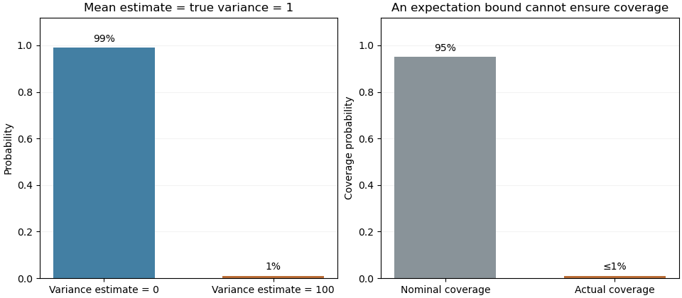
This example concerns the logical strength of the expectation criterion. Controlling the distribution of an estimated standard error, for example through an appropriate consistent estimator in an asymptotic argument, is additional work needed to justify confidence interval coverage.

Iduronic acid is a uronic acid found especially as L-iduronic-acid residues in dermatan sulfate and heparin. The neutral free acid has molecular formula ${\mathrm{C}}_6{\mathrm{H}}_{10}{\mathrm{O}}_7$; loss of its carboxyl proton gives iduronate.^[ref]

The biologically important L form differs from D-glucuronic acid at carbon 5. This epimerization changes stereochemistry while preserving the elemental composition. In a heparin-related biosynthetic reaction, heparosan-N-sulfate-glucuronate 5-epimerase converts D-glucuronate residues already present in a polymer into L-iduronate residues.^[ref]

For a hypothetical polymer segment containing ten eligible uronic-acid residues, conversion of three produces seven remaining glucuronate residues and three iduronate residues. The segment still has ten uronic-acid residues; chemical modification has changed their identities without adding three new sugar units. This is a distinction between modifying a chain and extending it.

Substrate context matters experimentally. The official enzyme record specifies a requirement for neighboring N-sulfated sugar residues and restrictions associated with O-sulfation. Supplying the free sugar alone therefore does not reproduce the stated polymer reaction.^[ref]

Actuator lag is delayed adjustment of an actuator's actual output to its commanded value. A simple dynamic model iswhere $u_{\mathrm{cmd}}$ is the command, $u$ the delivered quantity, $K$ the steady-state conversion and $\tau$ the time constant. A first-order actuator model with an estimated time constant appears in MathWorks's aircraft-parameter estimation example.^[ref]

For a step command of amplitude $U$ from zero initial output,The response reaches about63.2percent of its final value at one time constant and95.0percent at three time constants. In an original example with $K=1$, $U=10$ output units and $\tau =0.20\mathrm{s}$, the delivered value at0.20seconds is6.32, and its95percent rise takes about0.599seconds. The command itself has already reached10 at time zero.

The same model's frequency response is $K/(1+i\omega \tau )$. At $\omega \tau =1$, its magnitude is $|K|/\sqrt{2}$ and its phase lag is45degrees for positive $K$. Thus an actuator that is accurate for a constant command can still attenuate and phase-shift a rapidly changing command.

A direct identification experiment records the command and the actual output on a shared time base, applies a small step around an operating point, and estimates the final change and time to63.2percent. This is an explanatory procedure for the model, not a claim about a particular measured actuator. Sensor filtering, delay and an unknown initial state can alter the fitted response and must be included when relevant.

In a control system, treating $u=u_{\mathrm{cmd}}$ discards this state. The example in unmodeled dynamics shows how doing so changes closed-loop motion from a single exponential to a damped oscillation. Physical actuator saturation and rate limits are additional effects; the linear first-order lag equation does not represent them automatically.

A cuboctahedron is a convex uniform polyhedron with eight equilateral triangular faces and six square faces. Around each of its twelve vertices the faces alternate triangle, square, triangle, square. It has twenty-four edges, and the Euler characteristic check is $12-24+14=2$.

A concrete model is the convex hull of all coordinate permutations of $(\pm 1,\pm 1,0)$. The six planes $x=\pm 1$, $y=\pm 1$, $z=\pm 1$ cut out the square faces; the eight planes $\pm x\pm y\pm z=2$ cut out the triangular faces. All edges have length $\sqrt{2}$. Equivalently, join the midpoints of neighbouring edges of a cube: its vertices become triangular faces, and its faces become squares. The construction makes the name and the shared symmetries with the cube and octahedron visible.

Observation-time dependence of apparent compliance is the change in an inferred volume-per-pressure response when the measurement is made at different stages of filling or relaxation. For an original single passive compartment exposed to a pressure step,The equilibrium compliance is $C$, but a finite-time observation is smaller whenever $T$ and $\tau$ are positive and finite. A short observation can therefore confound stiffness with slow filling.

Two observation times identify the parameters only within the assumed model. Taking measurements at $T$ and $2T$ and defining $r=A(2T)/A(T)$ givesFor stipulated $A(1\mathrm{s})=0.10$ and $A(2\mathrm{s})=0.15\mathrm{L}(\mathrm{cm}{\mathrm{H}}_2\mathrm{O}{)}^{-1}$, this model gives $C=0.20$ and $\tau =1/\log 2\approx 1.44$ s. The parameter values follow from the model as well as the data.

A second original example exposes finite-time ambiguity between stiffness and slow filling. Suppose the real response is the sum of two compartments, each with compliance 0.10, but time constants 0.2 and 2 s. Then $A(0.5\mathrm{s})\approx 0.11391$ and $A(1\mathrm{s})\approx 0.13867$. Fitting the single-compartment formulas to just those two values gives $\tau \approx 0.328$ s and equilibrium compliance about 0.146, although the actual equilibrium sum is 0.20. Two exact measurements can fit the wrong model exactly.

Even one perfect finite-time value supplies no finite upper bound on equilibrium compliance without further restrictions. For an observed $A>0$ at time $T$, every choice $C>A$ can reproduce it withIncreasing compliance while increasing the filling time can preserve the measured response. Additional times, an independently bounded time scale or a validated compartment model add information.

The primary pilot study's discussion of non-uniexponential deflation and multiple time constants illustrates the experimental importance of this distinction.^[ref] The constructed calculations here are pressure-step examples, not patient measurements or a replacement for the study's actual compliance definitions.

Noncommuting damping and observation-time limits at resonance means that the late-time approximation of a damped circuit is not uniform as its dissipation tends to zero. A precise comparison needs an observable: the unnormalized resonant sinusoid itself has no ordinary limit as time tends to infinity. Use the series RLC circuit with zero initial conditions, source $V_0\cos {\omega }_{0}t$, and ${\omega }_0=1/\sqrt{LC}$. For $R>0$, its steady-state electric charge and electric current areThe remaining electrical resistance sets the resonant amplitude, as in the DOE series-resonance model.^[ref]

Define a dimensionless state error relative to that amplitude:For each fixed $R>0$, the homogeneous solution decays and $D_R(t)\to 0$. Conversely, on a fixed finite observation interval the actual circuit solution converges to the finite undamped solution as $R\downarrow 0$. The two terms containing $R$ then vanish, giving $D_R(t)\to 1$. Thus the genuine iterated limits areThis states the failure without treating an oscillating quantity as though it had a time limit.

For weak damping, put $\gamma =R/(2L)$ and ${\omega }_d=\sqrt{{\omega }_0^2-{\gamma }^2}$. The exact zero-state chargeboth verifies the decaying transient and recovers the undamped resonant response in undamped resonant forcing has no bounded sinusoidal steady state by a fixed-time expansion.

For an original timing comparison, $L=10\mathrm{mH}$ gives envelope decay times $2L/R=0.1\mathrm{s}$ at $R=0.2\Omega$ and $1\mathrm{s}$ at $R=0.02\Omega$. At a fixed $50\mathrm{ms}$ the respective exponential multipliers are about $0.607$ and $0.951$. A smaller electrical resistance can make the sinusoidal late-time approximation worse over a fixed acquisition window. MIT's steady-state notes explicitly require the startup transient to have disappeared.^[ref]

The U6 metal rescue experiment tests whether chemical groups in U6 small nuclear RNA position metal ions needed for RNA splicing. Its central perturbation is a phosphorothioate substitution: replace a selected non-bridging phosphate oxygen by sulfur. Changing the metal then tests whether altered ligand–metal compatibility can explain the resulting defect. This is a chemical interaction test within the assembled spliceosome.

In the 2013 yeast study, researchers introduced individual sulfur substitutions at twenty U6 positions. They activated and affinity-purified spliceosomes, then assayed their chemical reactions without ATP and soluble factors. This separated the assay from ATP-dependent activation and competing proofreading. Five tested substitutions strongly impaired branch formation in magnesium; cadmium supported rescue of branching. Exon-ligation rescue differed between substitutions, so rescue was not an interchangeable property of every altered phosphate.^[ref]

An original way to quantify the control logic is a ratio of ratios. Let $v_{O,A}$ and $v_{S,A}$ be measured activities for oxygen- and sulfur-containing RNA in metal A, with analogous values for metal B. Definewhen all denominators are positive. If switching metals multiplies every activity by the same amount, then $R=1$. Invented values $v_{O,A}=1$, $v_{S,A}=0.1$, $v_{O,B}=0.5$, $v_{S,B}=0.4$ give $R=8$: B preferentially relieves the sulfur-associated defect. This is an interaction metric, not a measured value from the paper or a direct metal-binding constant.

A preferential rescue still needs controls for folding, assembly and which reaction is being measured. The experiment's strength is connecting a particular RNA chemical group to catalytic output through a compensating perturbation. Omitting ATP after activation does not show that the complete cellular splicing process requires no ATP.

The halfspace depth of $x\in {\mathbb{R}}^d$ for a probability measure $P$ is the least mass of any closed half-space containing $x$:For an empirical distribution, it is the smallest fraction of observations in such a closed half-space. The boundary is included, so observations exactly on it count.

In one dimension,For observations $0,1,2$, the depth at $1$ is $2/3$, and the depth at either endpoint is $1/3$. Atoms can therefore give depth greater than $1/2$. An invertible affine map preserves halfspace depth, because it carries the family of closed half-spaces bijectively to itself and preserves their associated probabilities. A Tukey median maximizes this depth; the maximizing point need not be unique.

A Hermite-Gaussian optical mode is a separable paraxial field pattern whose transverse dependence is a product of Hermite polynomials and a Gaussian beam envelope. In an ideal aligned optical resonator with suitable spherical mirrors, these patterns form a family of transverse optical cavity modes. The two nonnegative integer orders $m,n$ count the straight nodal lines along the chosen transverse axes. The primary photonics notes give the mode fields and their order-dependent phase advance.^[ref]

At a common waist plane, choose a unit-normalized scalar fieldHere $H_j$ uses the physicists' Hermite polynomial convention, with $H_0(s)=1$, $H_1(s)=2s$ and $H_2(s)=4s^2-2$. The normalization follows fromAfter the two coordinate substitutions, $\iint u_{mn}^{\ast }{u}_{pq}dxdy={\delta }_{mp}{\delta }_{nq}$. Thus coefficients in a common-plane expansion can be recovered by inner products; the modes are orthogonal field patterns, not independent bright spots.

For $(m,n)=(1,0)$, intensity is proportional to $x^2{e}^{-2(x^2+y^2)/w_0^2}$, so its maxima lie at $x=\pm w_0/\sqrt{2}$, $y=0$. At $w_0=100\mu \mathrm{m}$, the bright lobes are about $141.4\mu \mathrm{m}$ apart. The field changes sign across $x=0$, although an intensity camera records positive intensity on both sides. For $(2,0)$, the nodal lines instead lie at $x=\pm w_0/2$. These patterns are illustrated in transverse optical cavity mode using individually peak-normalized images; equal peak intensity is different from equal integrated power.

A second-moment width of a Hermite-Gaussian optical mode distinguishes these multi-lobed beams quantitatively. Applying the Hermite polynomial recurrence inside the normalized integrals givesFor order $(1,0)$, the RMS widths are $\sqrt{3}{w}_0/2$ horizontally and $w_0/2$ vertically, despite the same envelope parameter $w_0$. Reporting a fitted single-lobe radius without its definition can obscure this difference.

During propagation the beam radius and wavefront curvature evolve, and the Gouy phase is multiplied by $m+n+1$. Consequently, transverse order contributes to the resonator's frequency condition and to confocal transverse-mode degeneracy. A proposed experiment scans the resonator while imaging a specified plane, then interferes its output with a reference field to test the phase reversal across a node. An intensity fit alone does not establish a pure coherent mode: mixtures, astigmatism, finite apertures and degeneracy can alter what is observed.

A square-tiled surface is a connected translation surface built by gluing finitely many equal Euclidean squares along paired parallel edges by translations. After normalizing side length to one, its area is the number of squares. Vertex identifications can create cone singularities with angle $2\pi k$ for a positive integer $k$.

Taking local square coordinates modulo ${\mathbb{Z}}^2$ gives a finite map to the flat torus ${\mathbb{R}}^2/{\mathbb{Z}}^2$. It is a translation covering away from the images of square vertices, with possible branching over the torus origin. Its degree equals the number of squares.

One square with opposite edges identified gives the ordinary flat torus. Two adjacent unit squares forming a $2$-by-$1$ rectangle, with opposite rectangle edges identified, give another flat torus and a degree-two unbranched map to the unit torus. More elaborate vertex gluings produce higher-genus surfaces. This gives a finite combinatorial encoding of examples used in flat geometry and dynamics.

The lac repressor, also called LacI, is the regulatory protein that reduces transcription of the lac operon by binding a lac operator in Escherichia coli. Binding of a small-molecule inducer changes the repressor's regulatory state through allostery. Allolactose connects this switch with lactose metabolism, while IPTG supplies an experimentally useful inducer. The lac repressor is distinct from the operator DNA and from the RNA polymerase whose transcriptional output is controlled.

Walter Gilbert and Benno Müller-Hill's 1966 isolation experiment gave the proposed regulator a biochemical measurement. Their equilibrium dialysis assay used radioactive IPTG: small free inducer could cross the membrane, while the macromolecular binding component was retained. Extra total labelled inducer on the protein side reported binding. The assay deliberately used inducer recognition rather than assuming that the exact mechanism of transcriptional repression was already established.^[ref]

An original one-site binding model explains that readout. If the free inducer concentration is $I$, the concentration of independent binding sites is $B_T$ and the dissociation constant is $K_I$, the bound concentration isAt equilibrium dialysis with matched solvent conditions, the protein side contains free plus bound inducer, $I+B$, while the opposite side contains free inducer $I$. Choosing $B_T=2\mu \mathrm{M}$ and $I=K_I=1\mu \mathrm{M}$ gives $B=1\mu \mathrm{M}$ and total concentrations $2$ versus $1\mu \mathrm{M}$. Equality of the free concentration does not require equality of the total concentration. The numbers are illustrative; the native lac repressor has a more detailed oligomeric and allosteric structure.

A separate one-operator model connects binding to expression. If a concentration $R$ of binding-competent repressor occupies the lac operator with probability $\theta =R/(K_O+R)$, and occupied DNA produces no transcripts in this model, thenReducing $R/K_O$ from $9$ to $1$ raises the model's transcription rate from $0.1r_0$ to $0.5r_0$. It does not follow that every measured cellular response obeys this one-site expression: operator arrangement, additional regulators and the later stages of gene expression affect the output. Measuring inducer binding and measuring repression therefore test related but different parts of the mechanism.

The repressor controlling the lac operon. Operator binding represses transcription, while inducer binding shifts the conformational equilibrium towards lower operator occupancy.

A torus factor of a toric variety is a product factor ${\mathbb{G}}_m^r$ in a toric decomposition $X\cong Y\times {\mathbb{G}}_m^r$. A nontrivial factor has $r>0$. This is stronger than merely containing a dense torus, which every toric variety does.

For a toric fan $\Sigma$ in a lattice $N$, let $N^{\prime }=N\cap {\mathrm{span}}_{\mathbb{R}}({\bigcup }_{\sigma \in \Sigma }\sigma )$. It is a saturated sublattice. Choosing a complementary lattice $N^{\prime \prime }$ givesThe complementary splitting need not be canonical. Thus a proper linear span of the whole fan supplies a nontrivial torus factor.

For the fan consisting of one coordinate ray and zero in ${\mathbb{Z}}^2$, the affine coordinate ring is $k[x,y,y^{-1}]$, giving ${\mathbb{A}}^1\times {\mathbb{G}}_m$. This variety has no torus-fixed point because the second multiplicative coordinate cannot be fixed by every scaling. A fan with only lower-dimensional cones can still span the whole lattice, so absence of full-dimensional individual cones alone does not imply a torus factor.