A feasibility threshold for averaging under shared uncertainty is the smallest uncertainty that repetition can approach while a common uncertain contribution remains unchanged. In the measurement model $X_i=S+D+{ϵ}_i$, suppose the shared term has variance ${\tau }^2$ and independent repeat noise has variance ${\sigma }^2$. ThenFor $\sigma >0$, every finite repeat count has $u_n>\tau$, although $u_n$ tends to $\tau$ as $n$ grows. A target below the floor is infeasible within this model, and a target exactly at it needs an infinite count. The GUM's correlated-input propagation explains why a common contribution is retained rather than divided by the repeat count.^[ref]

Approaching the floor has a quantifiable cost. To obtain $u_n\le \tau (1+\delta )$ with $\tau >0$, solveFor small positive $\delta$, the required count grows approximately as $1/\delta$. With stipulated $\sigma =0.04{\mathrm{m}}^2$ and $\tau =0.08{\mathrm{m}}^2$, getting within 1% of the floor needs 13 repeats, within 0.1% needs 125, and within 0.01% needs 1,250. These are planning examples for body surface area prediction, not observed clinical performance limits.

Precision limits of weighting correlated repeats show why a clever average cannot remove the common term for free. A linear estimate $\hat{S}={\sum }_i{w}_i{X}_i$ that preserves the unknown $S$ requires ${\sum }_i{w}_i=1$. The shared discrepancy therefore enters with coefficient one as well, givingThe inequality follows from ${\sum }_i{w}_i^2\ge 1/n$; equal weights attain it under the stipulated equal independent repeat-noise variances. Negative weights do not evade the floor while preserving the signal coefficient.

Reaching a lower uncertainty requires additional information or a changed measurement model that reduces the common contribution. Repeating a validation method with genuinely independent reference errors can supply different information, whereas repeating one person's height and mass measurements does not redraw that person's model discrepancy. A known bias calls for a correction, not a claim that averaging will make it disappear.^[ref]

The remaining-life validation cutoff is the information boundary used when reconstructing a forecast of remaining useful life at a particular issue time. Observations available by that time can enter the forecast; subsequent observations can establish the eventual end-of-life criterion crossing for scoring it. Keeping these roles separate prevents data leakage from turning a retrospective calculation into an apparently successful prediction.

For an original example, suppose a test reaches its specified endpoint at cycle100 and a forecast is evaluated as if issued at cycle60. The reference remaining life is40 cycles, known only after observing the later endpoint. Constructing a predictor that returns $100-t$ because the complete test record already reveals100 produces zero remaining-life validation error by construction. That is not evidence that the endpoint was predictable from the first60 cycles.

Preprocessing has the same information constraint. A trailing three-sample average $z_t=(x_{t-2}+x_{t-1}+x_t)/3$ uses observations available at $t$. A centered average $z_t^{\prime }=(x_{t-1}+x_t+x_{t+1})/3$ needs a future observation. The centered average can be legitimate with a declared one-sample reporting delay, but then its forecast issue time is $t+1$, not $t$. Parameter fitting, normalization and selection among candidate models also belong inside the information boundary.

NASA's battery-aging records provide a physical example of the required distinction: they contain measured discharge current, terminal potential and temperature, together with a capacity-loss aging endpoint and run-to-failure histories.^[ref] A validation experiment can reveal only the prefix through its chosen cutoff to a prediction method, save the forecast, and subsequently compare it with the endpoint in the withheld suffix.

A fixed model trained on other complete histories can be evaluated on a new component's prefix. A method that updates online must instead document which new observations have become available before each forecast. In either case, preserving the cutoff, endpoint definition and assumptions about future operation makes the resulting remaining-life validation error interpretable. Pooling all prediction times into one score can conceal a violation at a particular cutoff.

For a nonzero reference transfer function $H_{\mathrm{ref}}$, the complex relative gain error is the relative errorIt measures the distance from the complex ratio to one, so it responds to both amplitude error and phase error. A vector vector network analyzer measures both quantities; replacing its complex result by a magnitude discards part of the measured information.^[ref]

Write $H/H_{\mathrm{ref}}=a{e}^{i\varphi }$, where $a\ge 0$ and $\varphi$ is the phase difference. Multiplying by the complex conjugate givesThus a pure five-degree phase error has $E=2\sin (2.5\pi /180)\approx 0.08724$, about $8.72\%$, even though the magnitude ratio is exactly one. For small $\delta =a-1$ and small $\varphi$ measured in radians, $E\approx \sqrt{{\delta }^2+{\varphi }^2}$. Adding the two unsigned errors is generally not the same operation.

The metric also controls signals. Suppose two linear time-invariant systems have frequency responses $H,H_{\mathrm{ref}}$ and act on the same input in L2 space. On its frequency support assume $H_{\mathrm{ref}}\ne 0$ almost everywhere and $|H/H_{\mathrm{ref}}-1|\le \epsilon$ almost everywhere. Applying the norm bound for a Fourier multiplier on L2 to the reference output yieldsThis is an output-relative bound, so input frequencies suppressed by a zero of $H_{\mathrm{ref}}$ require separate treatment. Near a reference zero, a small absolute error can produce an enormous complex relative error; an absolute or explicitly fixed-scale tolerance is then more informative.

A model of a regularity structure realizes the abstract symbols of a regularity structure $(A,T,G)$ as concrete distributions, consistently across expansion points. It comprises continuous linear realization maps ${\Pi }_x:T\to {\mathcal{S}}^{\prime }({\mathbb{R}}^d)$ and maps ${\Gamma }_{xy}\in G$ satisfyingThus ${\Gamma }_{xy}$ transports an expansion from $y$ to $x$ without changing the represented distribution.^[ref]

Analytic bounds connect each symbol's assigned order $\alpha$ to its actual small-scale size. For ordinary isotropic scaling, put ${\phi }_x^{\lambda }(z)={\lambda }^{-d}\phi ((z-x)/\lambda )$. For $\tau \in T_{\alpha }$ one requiresThese bounds are uniform on each compact set of base points, below each fixed upper order, for $0<\lambda \le 1$ and smooth test functions supported in the unit ball with $C^r$ norm at most one; choose an integer $r>\max (0,-\inf A)$. Other scaling choices change the rescaled test functions and distance. Negative $\alpha$ allows singular distributions, whose small-scale averages can grow as $\lambda$ shrinks.^[ref]

In the one-dimensional polynomial model of a regularity structure, $({\Pi }_x{X}^n)(z)=(z-x{)}^n$ and ${\Gamma }_{xy}X=X+x-y$. For $x=1,y=2$,A change of variable $z=x+\lambda w$ in the test function pairing gives exactly ${\lambda }^n\int w^n\phi (w)dw$, explaining the analytic bound for the monomial $X^n$. The realization maps supply information absent from the abstract triple alone.

A strict record in a sequence $X_1,X_2,\dots$ occurs at index $n\ge 2$ when $X_n>\max \{X_1,\dots ,X_{n-1}\}$. The first observation is conventionally a strict record. A tie with the previous maximum is excluded: the observations $3,3,4,2,5$ have strict records at indices $1,3,5$.

If the observations are independent and identically distributed with a continuous cumulative distribution function, their maximum among the first $n$ observations is unique almost surely. By exchangeability, each of the $n$ positions has the same probability of containing that maximum. Thus the probability of a strict record at $n$ is $1/n$, and linearity of expectation gives an expected number ${\sum }_{j=1}^{n}1/j$ of strict records up to $n$. Ties or dependence can change the calculation; identical marginal probability distributions alone do not justify the symmetry argument.

Jamming in random sequential adsorption occurs when previously accepted objects leave no permitted position for another object. The placement rule is irreversible: an object that would overlap an accepted object is rejected, and accepted objects are not rearranged. A jammed configuration need not have the greatest possible covered fraction.

For a one-dimensional example in which touching endpoints is allowed but overlapping interiors are forbidden, place unit intervals $[0.5,1.5]$ and $[1.6,2.6]$ inside $[0,3]$. The uncovered gaps have lengths $0.5$, $0.1$ and $0.4$. No gap can contain another unit interval, so the configuration is jammed even though only $2/3$ of the containing interval is covered. Three unit intervals could cover it completely under a different placement history. This is the geometric obstruction modeled by irreversible parking in random sequential adsorption; the final coverage depends on the proposal rule and object geometry, rather than on a universal packing fraction.

Femtosecond stimulated Raman spectroscopy, or FSRS, measures a Raman spectrum through gain induced in a short broadband probe by a narrowband Raman pump. At a molecular vibration frequency matching the pump–probe frequency difference, Stokes Raman scattering transfers energy from the pump into the probe. The narrow pump and spectrograph supply spectral selectivity while the short probe samples the system in time; the probe duration alone is not the spectral linewidth.^[ref]

The2003 apparatus of David W. McCamant, Philipp Kukura and Richard A. Mathies filtered a Ti:sapphire amplifier output to make a narrowband pump near $793\mathrm{nm}$ and generated a broadband probe in sapphire. Overlapped beams traversed the sample; a spectrograph dispersed probe and reference spectra onto a dual-diode array. The paper demonstrates gain bands in cyclohexane.^[ref]

After dark correction, let $S$ and $R$ denote probe and reference counts. The Raman pump-on pump-off gain ratio isFor an original chosen spectral channel, take $(S,R{)}_{\mathrm{off}}=(10000,10000)$ and $(S,R{)}_{\mathrm{on}}=(11440,11000)$. The normalized ratio is $1.04$, a four-percent Raman gain; the unnormalized probe ratio $1.144$ would mistake a source fluctuation for additional gain. This assumes a linear detector and a reference that tracks that fluctuation.

A second original calculation uses an $800\mathrm{nm}$ pump and a $1000\mathrm{c}{\mathrm{m}}^{-1}$ vibration. The Stokes probe channel is at wavenumber $12500-1000=11500\mathrm{c}{\mathrm{m}}^{-1}$, or about $869.6\mathrm{nm}$. A broadband probe can sample many such differences simultaneously. Spatial and temporal overlap, wavelength calibration, probe chirp and non-Raman nonlinear backgrounds still require characterization. A short pulse label does not by itself establish the time resolution of a changing molecular response.

Spatially offset Raman spectroscopy, or SORS, collects Raman scattering from a surface region laterally displaced from the illumination spot. In a diffusely scattering material, changing the offset changes the mixture of photon paths and the relative contributions of surface and buried layers. It is not simply a tightly focused measurement at a selected depth.

The2005 experiment of P. Matousek and colleagues used trans-Stilbene powder beneath a $1\mathrm{mm}$ layer of PMMA powder. Its primary report describes a19-fold improvement in buried-layer contrast before numerical separation.^[ref] The physical point is that an opaque-looking scattering overlayer need not contribute the same spectral proportion at every collection offset.

An original two-component linear combination illustrates scaled subtraction of two spatially offset Raman spectra. Let $S(\nu )$ and $B(\nu )$ be fixed surface and buried Raman spectra, and suppose dark-corrected measurements giveIf a surface-specific band determines the scale $3/8$, thenThe surface contribution cancels while a scaled buried spectrum remains. These coefficients are chosen examples, not the paper's measured mixing fractions.

A practical arrangement fixes an excitation spot, moves the collection region laterally, rejects the excitation line with an optical filter, and sends the collected light to a spectrograph. Record comparable exposure, incident radiant power, backgrounds and spectral response at each offset. If the offset changes each component's shape, rather than only its scale, the simple subtraction model fails. Strong absorption, fluorescence, overlapping bands and measurement noise also limit inference. Offset-dependent enrichment provides evidence for depth-dependent contributions; it is not an unqualified depth calibration or unique chemical identification.

A Raman spectrum records the strength of Raman scattering as a function of scattered optical frequency or, usually, Raman shift relative to the excitation. For vacuum wavelengths in nanometres, a common wavenumber convention isHere the numerical wavelengths are in nanometres. Stokes Raman scattering has positive shift under this convention; Anti-Stokes Raman scattering has negative shift. The strong unshifted Rayleigh scattering line is not a vibrational Raman band.

For an original chosen excitation ${\lambda }_0=500\mathrm{nm}$ and a $1500\mathrm{c}{\mathrm{m}}^{-1}$ vibration, the Stokes wavenumber is $20000-1500=18500\mathrm{c}{\mathrm{m}}^{-1}$, giving ${\lambda }_s\approx 540.54\mathrm{nm}$. The corresponding anti-Stokes wavelength is $10^7/21500\approx 465.12\mathrm{nm}$. Changing the excitation changes these optical wavelengths while the same assumed transition retains its Raman shift. The One-mode Raman spectrum example gives an existing level diagram and a separate numerical spectrum.

The vertical quantity must be stated too: detector counts per spectral bin, calibrated scattered power density and a stimulated gain ratio are different observables. Femtosecond stimulated Raman spectroscopy can plot the Raman pump-on pump-off gain ratio rather than spontaneous photon counts. Its primary apparatus disperses probe and reference beams onto an array and calibrates shifts with known solvent lines.^[ref]

Spectral-density conversion between wavelength and Raman shift also changes the density's units: rebadging the horizontal axis alone need not preserve a spectral integral. Background, excitation rejection, instrument response and spectral resolution affect observed band heights and widths. An integrated band area is not determined by peak height alone. A chemical inference should compare calibrated positions and responses under specified conditions, rather than identify a material from one unqualified peak.

A Raman shift as a probe of bond stiffness interprets a measured vibrational frequency through a mechanical model of the assigned mode. For one stretching coordinate modeled as a harmonic oscillator,where $k_{\mathrm{eff}}$ is an effective spring constant and ${\mu }_{\mathrm{eff}}$ an effective mass. For an isolated diatomic stretch the latter is the reduced mass. A collective normal mode can involve many atoms, so its effective stiffness is not automatically the force constant of one selected bond.

An original same-mode example shifts from $1500$ to $1530\mathrm{c}{\mathrm{m}}^{-1}$. If the effective mass is unchanged, the harmonic model givesor a $4.04\%$ increase in effective stiffness. The small-change version isA ten-percent mass increase at fixed stiffness would instead reduce the frequency by $1/\sqrt{1.10}\approx 0.9535$. This reduced-mass ambiguity in a Raman stiffness inference is why a frequency change alone does not uniquely measure a stiffness change.

Mechanical strain can shift Raman bands by changing the local vibrational dynamics. HORIBA's application documentation illustrates stress mapping in microfabricated silicon, including shallow-trench regions, and describes a correlation between applied stress and peak shift.^[ref] That calibrated material response is more specific than treating every shift as a direct scalar bond-stiffness measurement.

A motivating experiment would track the same assigned band while varying a known load, holding temperature, excitation and polarization conditions fixed and measuring the wavelength reference. Heating, isotopic composition, mode mixing and structural changes can also alter frequencies. The Raman shift gives an energy spacing; mechanical interpretation additionally needs the mode assignment, mass model and appropriate stress/strain calibration.

Raman mapping records Raman spectra at known sample positions and constructs spatial maps from their spectral features. A map can show composition or structural variation that is absent from an ordinary reflected-light image. A point-scanning apparatus combines a focused laser, microscope objective, rejection of unshifted light, a spectrometer and controlled sample positioning. A primary university facility description identifies single-point acquisition and two-dimensional mapping as measurement modes.^[ref]

The acquired data can be represented as $I(x,y,\tilde{\nu })$, with position coordinates $x,y$ and Raman shift $\tilde{\nu }$. It is a form of hyperspectral imaging. The displayed image is a derived summary of those spectra. For example, a baseline-corrected Raman band-area map useswhile a Raman peak-position map records a fitted band's position. Different summaries can reveal different properties of the same sample. Manufacturer examples include a silicon-carbide wafer whose spectral map separates inclusions and structural variation.^[ref]

For an illustrative20µm-by20µm point map sampled every1µm with both boundaries included, there are $21\times 21=441$ positions. At0.10s exposure per position, exposure time alone is44.1s; motion and readout add overhead. Reducing step size increases sampling density, while optical resolution remains constrained by the excitation/detection point spread function and instrument configuration. A finely interpolated display cannot recover an unsampled small inclusion.

Intensity also depends on illumination, focus and the spectral background. A single-frequency brightness map can mix a desired Raman band with broad background, whereas fitted or integrated features can answer a more specific question. Quantitative composition or stress estimates require an appropriate measurement calibration; a colourful spatial contrast is not by itself a calibrated concentration or stress measurement.^[ref]

Uncollected scattering in a radiometric energy balance is outgoing scattered radiation that falls outside the measured channels. Assigning every missing joule to optical absorption then overestimates the absorbed energy. The radiometric energy balance must count disjoint transmitted, reflected, scattered and absorbed terms for the same interval.

For an original collection model, stipulate $100\mu \mathrm{J}$ incident, $30\mu \mathrm{J}$ transmitted and $20\mu \mathrm{J}$ specularly reflected. A separate scattered-light receiver collects $q=10\mu \mathrm{J}$. If its calibrated capture fraction is $c=0.25$, the scattered energy is $q/c=40\mu \mathrm{J}$, leaving $10\mu \mathrm{J}$ absorbed. If all that is known is $0.20\le c\le 0.50$, scattering can range from $20$ to $50\mu \mathrm{J}$ and absorption from $0$ to $30\mu \mathrm{J}$. One receiver reading cannot determine both the total scattering and its capture fraction.

The fraction $c$ is an energy fraction, not automatically the receiver's fraction of solid angle. Converting geometrical coverage into an energy fraction also needs the scattering distribution.

An integrating sphere provides broad angular collection through repeated diffuse reflection. Actual reflectance/transmittance arrangements depend on port geometry, baffles and whether the specular component is included. The primary guide describes excluding that component through a port and using baffles to prevent direct viewing of the illuminated sample.^[ref] The apparatus therefore needs its own response calibration; calling a receiver integrating does not establish perfect collection.

The encircled radiant energy of a Gaussian beam is the radiant energy inside a centred circular receiver at a specified transverse plane. For fixed Gaussian beam radius $w$ and total laser pulse energy $U$,The radiant exposure of a Gaussian beam contains the radial integration and aperture-capture plot. Its $w$ is the irradiance $e^{-2}$ radius, as specified in the primary beam account.^[ref]

An original annular example distinguishes energy near an axis from energy between two radii. Subtracting two encircled values givesChoose $U=5\mu \mathrm{J}$, $w=0.50\mathrm{mm}$, $R_1=0.25\mathrm{mm}$ and $R_2=0.50\mathrm{mm}$. The annulus receives $5(e^{-1/2}-e^{-2})\approx 2.356\mu \mathrm{J}$, or 47.12 percent of the full beam energy. A bright central point does not imply that most energy lies in an arbitrarily small disk around it.

Indeed, the radial radiant-energy density of a Gaussian beam is $dQ/dR=2\pi RH(R)$, where $H$ is local radiant exposure. For this profile it is largest at $R=w/2$, even though $H$ is largest at zero radius. Increasing a centred aperture and comparing integrated detector readings can test the cumulative prediction. Detector linearity, aperture alignment and the finite collection boundary must be controlled; a displaced aperture is not described by the centred formula.

The quotient map of vector spaces $\pi :V\to V/U$ sends a vector $v$ to its coset $v+U$, where $U$ is a linear subspace. It is a surjective linear map with kernel $U$: two vectors have the same image exactly when their difference lies in $U$.

For $V={\mathbb{R}}^2$ and $U=\mathrm{span}(1,0)$, the quotient retains only the second coordinate, so every horizontal line represents one quotient vector. More generally, a linear map $f:V\to W$ vanishing on $U$ factors uniquely as $f=\overline{f}\circ \pi$. The formula $\overline{f}(v+U)=f(v)$ is well defined because changing the representative by an element of $U$ leaves its value unchanged.

For a differentiable family of density matrices ${\rho }_{\theta }$, the symmetric logarithmic derivative is a Hermitian operator $L_{\theta }$ satisfyingIf ${\rho }_{\theta }={\sum }_j{p}_j|j⟩⟨j|$, its determined matrix entries are $(L_{\theta }{)}_{jk}=2⟨j|{\partial }_{\theta }{\rho }_{\theta }|k⟩/(p_j+p_k)$ whenever $p_j+p_k>0$. Entries wholly in the kernel are undetermined when a solution exists and do not affect $\mathrm{Tr}({\rho }_{\theta }{L}_{\theta }^2)$. Rank-changing boundary points need extra care.

For ${\rho }_{\theta }=\mathrm{diag}(\theta ,1-\theta )$, $0<\theta <1$, one gets $L_{\theta }=\mathrm{diag}(1/\theta ,-1/(1-\theta ))$ and Quantum Fisher information $F_Q=1/[\theta (1-\theta )]$. This recovers ordinary Fisher information for a binary observation. In noncommuting families the symmetrized equation supplies the operator version needed to quantify local sensitivity.^[ref]

Identifiability from linear observations asks which features of an unknown vector $\theta \in {\mathbb{R}}^p$ are fixed by observing $y=A\theta$. Two parameter vectors are observationally equivalent exactly when their difference lies in the kernel of a linear map $A$:Thus the full vector is identifiable precisely when $\ker A=\{0\}$, equivalently when $A$ has full column matrix rank. Repeating the same rows can improve precision in a noisy measurement without increasing this rank.

A linear target $g(\theta )=c^{\mathsf{T}}\theta$ requires less information. It is identifiable if and only if $c$ is in the row space of $A$. If $c=A^{\mathsf{T}}d$, then $g(\theta )=d^{\mathsf{T}}y$, so the target is recovered directly. Conversely, an identifiable target must vanish on every observationally invisible difference: $c^{\mathsf{T}}h=0$ for every $h\in \ker A$. Orthogonality to the kernel is exactly row-space membership. This is a concrete instance of quantity-specific identifiability; the primary identification literature also treats identification of individual parameter components by rank conditions.^[ref]

For an original example, supposeBoth $(1,4,3)$ and $(2,3,4)$ fit perfectly. Their difference is a multiple of $(1,-1,1)$, which spans the kernel. The target ${\theta }_1-{\theta }_3=y_1-y_2=-2$ is identified, whereas ${\theta }_1+{\theta }_2+{\theta }_3$ takes values 8 and 9 and is not. A new independent measurement of ${\theta }_2$ restores full identification; another copy of $y_1$ does not.

The same distinction applies to a statistical model $Y\sim N(A\theta ,\Sigma )$ with known positive-definite covariance matrix $\Sigma$: two parameters give the same observable law precisely when their means agree. A Moore-Penrose pseudoinverse selects one solution when the system is underdetermined, but that numerical convention does not show that the selected vector is the unique physical parameter. Additional restrictions must be justified as assumptions, not silently supplied by a solver.

The pulsed Doppler depth-velocity tradeoff is the restriction linking uniquely localized depth and unaliased beam velocity in a simple repeated-pulse Doppler ultrasound acquisition. Deeper echoes take longer to return, leaving fewer distinct pulse observations per second. Fewer observations reduce the unaliased Doppler ultrasound frequency interval.

For maximum depth $d$, speed of sound $c$ and pulse repetition frequency $f_r$, the ideal nonoverlapping timing restriction is $f_r\le c/(2d)$. The Nyquist frequency is $f_r/2$. Combining this with $f_D=2f_{0}v\cos \theta /c$ givesThe strict inequality excludes the ambiguous Nyquist endpoint. For beam-parallel motion, $|\cos \theta |=1$. At a right angle there is no first-order Doppler sensitivity to the motion; the apparent divergence of the formula does not provide unlimited useful velocity measurement.

For an original calculation, let $c=1540$ m/s and $f_0=2.5$ MHz. A 15 cm depth allows at most approximately 5133 pulses/s in this idealization, with axial Nyquist speed about 0.791 m/s. At 30 cm these bounds fall to approximately 2567 pulses/s and 0.395 m/s. Doubling the transmitted frequency to 5 MHz halves the axial velocity limits at either depth.

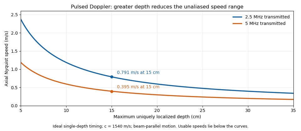
These are timing and sampling bounds, not a specification for a particular instrument. Pulse duration, scheduling and processing can lower the usable limit. Moving a spectral baseline changes the displayed signed interval but does not increase its total sampled-frequency width. Continuous-wave Doppler echocardiography avoids this pulse-rate restriction while sacrificing unique depth selection; high-pulse-rate acquisition instead accepts Doppler range ambiguity.^[ref] The acquisition choice determines which ambiguity remains.