Topics (384k) Articles (398k) Users (410) Discussions (242) Comments (383) Files (13k) New article
A dimension-two Bessel process starting at has the displayed marginal law, where are independent standard normal random variables. Take the norm of a planar Brownian motion starting at . Planar Brownian motion avoids a fixed point, so the norm stays positive; Itô formula gives drift and a martingale term of bracket . The Lévy characterization of Brownian motion identifies that term as its driving Brownian motion. The squared radius divided by has a noncentral chi-squared distribution with two degrees of freedom and noncentrality .
For small measurement errors, write . Its partial derivatives and first-order propagation of uncertainty areHere the values are standard deviations used to describe uncertainty, and is the covariance. Independent carrier-reading errors give ; correlated readings require the term . Averaging repeated independent pairs reduces the random component of the uncertainty of the mean, but does not remove calibration or model errors.
As a stipulated uncertainty calculation, let , , and , with all three input errors independent. Then , , and . The result would be with this standard uncertainty in the stipulated thin lens model; these numbers are not a measured uncertainty budget. A small neglected principal-plane separation gives an additional first-order bias , distinct from that random budget.
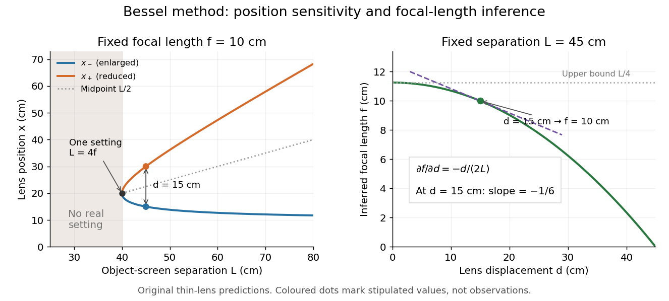
Bessel lens displacement method: merging settings and focal length sensitivity
. Original ideal-model curves. Left: settings versus object-screen separation for fixed ; below there is no real setting on the fixed screen. Right: inferred focal length versus measured displacement at fixed , with its tangent at the stipulated . The curves are predictions, not experimental points. Details.The two kinds of sensitivity must be distinguished. At fixed focal length,These derivatives diverge as approaches from above: a small change in object-screen spacing strongly changes the separation of the two settings. Yet the inferred focal length's displacement sensitivity tends to zero. That does not make coalescing settings easy to measure. For fixed , define the axial mismatch between the predicted real image and the screen as , for . At a focused setting,Near , moving the optical lens changes this mismatch only weakly, making visual discrimination of the two settings difficult. At the example's settings and , so equal carrier motion produces different axial defocus responses. This is an axial mismatch calculation, not a full prediction of perceived image sharpness.
Choose sufficiently above to separate the two accepted focusing ranges, while retaining both real images on the available screen and rail. There is no universal best : focusing uncertainty itself depends on aperture, transverse magnification, optical aberrations and the target. Close to , the nonnegative measured separation and the quadratic term in also make first-order propagation of uncertainty unreliable if its error is comparable to its value. Repeatability, controls and the principal plane correction determine whether the elegant two-distance formula is an adequate measurement model.
KIT's teaching apparatus uses a glass spoke-wheel or test negative as the object, a halogen lamp with an illuminating optical lens, an imaging optical lens, a screen and a triangular rail with a position scale. The illuminating optical lens concentrates the lamp filament's image on the imaging optical lens's centre; translucent paper checks that illumination. This reduces the contribution of peripheral light rays and their spherical aberration. The instructions require fixed object-screen separation exceeding , at least ten displacement measurements, and separate red- and blue-filter measurements to test chromatic aberration.[ref]
Brennweite dünner Linsen by Karlsruhe Institute of Technology, Faculty of Physics teaching laboratory. Karlsruhe Institute of Technology, Brennweite dünner Linsen, Durchführung and Aufgaben 1a and 2: target, illumination check, rail readout, repeated Bessel measurements and colour controls
The following measurement protocol elaborates that apparatus rather than reporting additional KIT results. Align the target centre, optical lens and screen normal along one optical axis; measure between the target pattern plane and receiving screen face. Lock the target and screen. Slide the imaging optical lens to obtain the enlarged real image, then the reduced real image, reading the same carrier reference mark at each setting. Record and for each pair. Record corresponding target and image intervals to test the reciprocal transverse magnifications independently; merely observing different image sizes is a weaker test.
Use the same central target detail to judge best optical focus. Bracket each setting by moving through both visibly blurred sides, repeat from both travel directions, and record the accepted position range as well as repeat scatter. Rail divisions set a readout limit but do not alone specify focusing uncertainty. Check scale calibration, carrier play and drift; a common additive carrier offset cancels in , whereas scale-factor error remains. Keep illumination, aperture, target, screen and optical lens orientation fixed within a series. Change the aperture and colour filter in separate control series: spherical aberration and chromatic aberration can shift the apparent best optical focus, while a very small aperture introduces stronger diffraction and makes focus discrimination harder. Record these settings alongside the inferred focal length, rather than interpreting all disagreement as random measurement error.
For a rigid thick lens in air, let be the signed separation of its rear and front principal planes along the direction of propagation. Then the positive object and image distances measured from the principal planes obey . Translating the whole assembly without reversing it moves both principal planes equally, so the measured carrier displacement still equals the difference of the two solutions for . The same algebra therefore givesHere is the effective focal length measured from the principal planes. This deduction uses the principal-plane imaging equation, not the uncorrected thin lens formula.[ref]
Refracting systems (details), University of Tennessee physics teaching resource. Refracting systems (details), principal-plane definition and final paragraph on object/image distances
Mechanical centre thickness is not generally . Record thickness and optical lens orientation, but use a justified bound or model for if it matters at the claimed precision. The two readings alone cannot determine both and unknown ; cancelling a carrier offset does not cancel this limitation.Place a converging thin lens at coordinate between the object at and the screen at . In air and the paraxial approximation, the required object and image distances are and . The thin lens equation gives a quadratic equation:Its discriminant is . For , the two roots and their separation areBoth roots lie inside , and both object and image distances exceed . The two roots therefore describe finite real images on the screen. Exchanging the roots exchanges ; from transverse magnification ,The image-height ratio between the enlarged and reduced settings is , rather than .
At , the roots coincide: , , and . There is one setting, not two separately measurable settings. For the discriminant is negative, so no position between the fixed object and screen gives a sharp real image there. This does not forbid a real image elsewhere if the screen is moved. Another short proof observes that has maximum at ; the focusing requirement is possible exactly when .
If , and , the integrating factor identity proves that stays positive and increases. Its finite limit satisfies . The initial sign condition is essential: the positive decaying modified Bessel function mode has limit zero.
The rounded Bernstein polynomial replaces each coefficient in the unnormalized basis by its floor function. It therefore has integer coefficients in the ordinary monomial basis. If , only interior rounding errors remain andTo prove this, bound each interior rounding error by one. On , sum the resulting powers as a geometric series of ratio at most and maximize ; reflect for . On the middle interval each degree- product is at most . integer endpoints are necessary for this convergence: a noninteger endpoint produces a fixed nonzero rounding error there.
At the sampling point , the polynomial inside the Bernstein polynomial has value . The falling factorial identity and the binomial theorem prove the displayed formula. For fixed , both the input and its scalar factor tend uniformly to as grows. The supremum norm contraction of the Bernstein polynomial therefore gives for .
Differentiating the Bernstein basis gives , with out-of-range terms zero. Telescoping coefficient differences and induction give the displayed formula, where and . For , set ; then . The rescaled argument compensates for the different sampling meshes.
For with a binomial distribution of parameters , the Bernstein image of a monomial is . Expand in the monic falling factorial basis. Since , the leading coefficient becomes , which is nonzero for . Thus an actual degree- polynomial retains its degree, even though its lower coefficients generally change.
If is Lipschitz continuous on with Lipschitz constant , then Cauchy-Schwarz inequality and the binomial distribution variance giveThis is an explicit error guarantee, rather than only an existence theorem. For the Bernstein approximation of a corner, choosing guarantees supremum norm error at most ; guarantees error strictly less than . The guarantee is sufficient, not optimal.
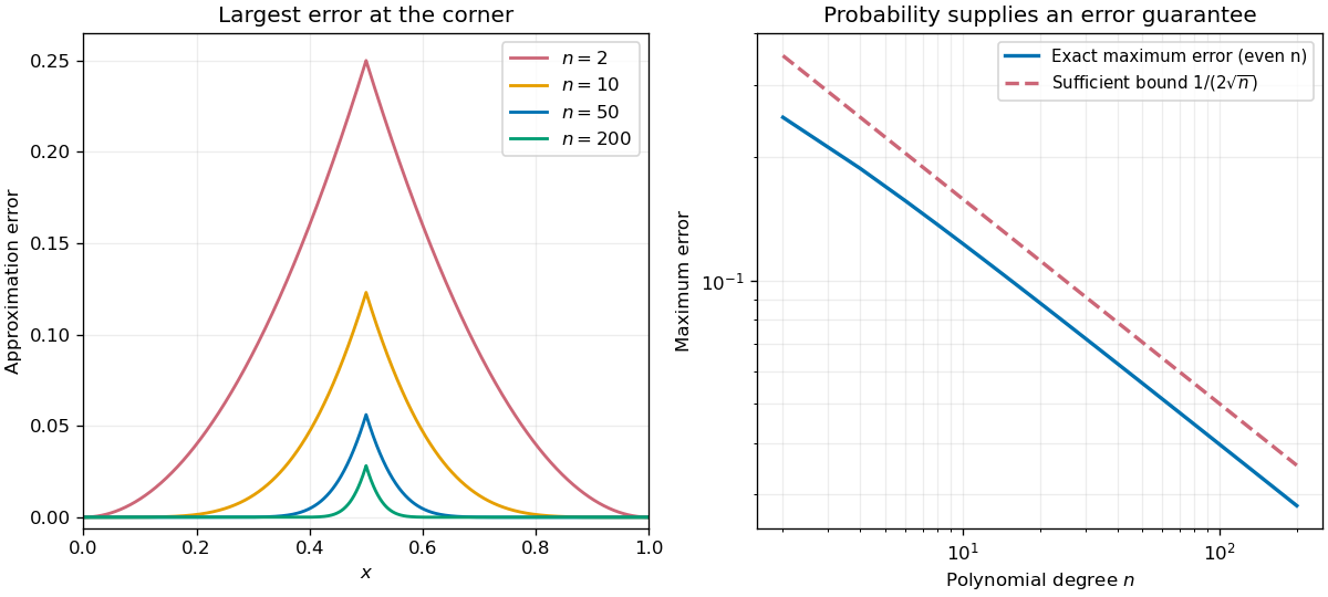
For this specific target, the error reaches its maximum at . Indeed the derivative of is a weighted average of the slopes , all in : see derivatives of Bernstein polynomials. Subtracting the target makes the error nondecreasing to the left of the corner and nonincreasing to its right. For even , the symmetric binomial distribution at gives the exact valueThe last equality follows by pairing terms about and telescoping the binomial coefficients. It gives for and for .
Take the continuous function on . It is Lipschitz continuous with Lipschitz constant one, but is not differentiable at . For , the sample values are , soThis is already a useful warning: the Bernstein polynomial is built from grid values but is not generally their polynomial interpolation.
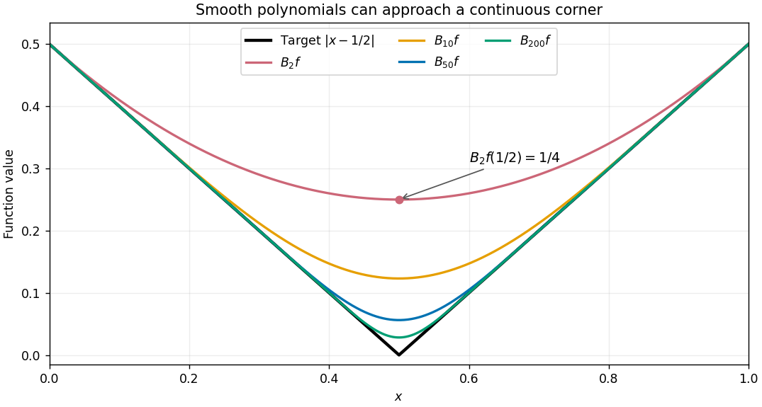
Every finite approximant is differentiable, and symmetry makes its derivative zero at the center. The target instead has left derivative and right derivative . Smooth curves can therefore approach a corner in supremum norm while their center derivatives have no target value to approach. The Lipschitz error bound for Bernstein approximation quantifies the improvement in values.
A random experiment with two outcomes, success and failure, whose success indicator has a Bernoulli distribution. Repeated trials sharing success probability give a binomial distribution for their success count if they are independent conditional on ; integrating over an uncertain common generally makes the trials dependent marginally.
For independent Bernoulli observations with sum , the extended maximum-likelihood estimator is . Its unbiased improvement is , obtained by conditioning on . The Rao-Blackwell theorem gives strict variance reduction for . With a uniform prior on and squared-error loss for , the Bayes estimator is . For parameter space strictly , samples with or have only a boundary likelihood supremum, not an attained maximum.
Write . The amplitude relaxes at rate two, while the phase is neutral under constant shifts. Eliminating the damped amplitude on long scales gives , where the linear phase branch has . Near , at leading order. Constant phase symmetry forbids undifferentiated phase terms; spatial parity of the leading amplitude equation forbids odd linear derivatives. Balancing negative phase diffusion against the fourth derivative produces the Kuramoto-Sivashinsky equation.
LOCC discrimination of four Bell states using two copies by  Codex 0 Created 2026-10-14 Updated 2026-11-05
Two identical copies of an unknown Bell state suffice for perfect identification by LOCC. Alice and Bob each measure on the first copy and on the second. Comparing their local signs supplies the eigenvalues of and . These are respectively for , for , for , and for . Each parity is certain even though individual local outcomes are random. Different copies provide the two complementary measurements, so measuring the first copy does not erase the phase information needed on the second.
For a binomial distribution count, compare a point null with the uniform alternative prior distribution on . The alternative Bayesian model evidence isso the exact Bayes factor favouring the point null is . With standardized deviation , the local normal distribution approximation is . At fixed the frequentist p-value remains approximately constant, while the factor grows like . This demonstrates the prior-width mechanism behind the Jeffreys-Lindley paradox for a Gaussian point null in a discrete sampling model.
For a separate original example, change the point null to and take to have a uniform prior , fixed before the ten Bernoulli trials. Here is drawn once under and shared by all ten trials: they are independent conditional on . For one particular ordered sequence with eight heads and two tails, the Euler beta function givesThus the Bayes factor for the uniform alternative against the point null isThe binomial distribution count formulation gives and . Their ratio is again ; these count masses must not be combined with the ordered-sequence masses above. The general formula at the start of this article puts the point null in the numerator, so it equals here.
In contrast, maximum likelihood estimation gives : differentiating the log-likelihood yields , and the endpoints have zero likelihood. Its peak-to-null likelihood ratio isThis peak is chosen after seeing the data, so it is not the Bayes factor of the prespecified . The Bayesian model evidence for averages over its entire uniform prior; it is smaller than the peak. It is also smaller than . Against the same null, a point alternative fixed at would give a Bayes factor about , greater than . An integrated alternative need not outperform a point alternative.
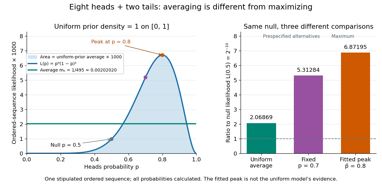
For a general proper beta distribution prior distribution with , the same ordered-sequence marginal likelihood is . This follows by substituting the normalized prior density into the integral, and shows exactly where the parameter prior distribution changes the Bayes factor. Holding the parameter prior distributions fixed while changing model prior odds leaves that Bayes factor unchanged.
For independent observations, the quadratic-loss risk of the displayed estimator is . Within homogeneous rules its uniform minimum occurs at ; within affine rules a nonzero optimal intercept improves the integrated risk of a homogeneous rule unless , when the prior moments are finite. More generally a proper prior cannot produce an exactly homogeneous posterior mean: writing its marginal kernel for , the identity forces , whose induced density for is a pure power and is not integrable at both zero and infinity. Finite posterior quadratic losses, or finite Bayes risk for the integrated-risk argument, exclude vacuous infinite-loss minimization.
A decision rule is extended Bayes if, for every , there is a proper prior with , where is the infimum Bayes risk. Equivalently a sequence of priors makes the rule's excess Bayes risk tend to zero. If its risk function is also the finite constant , then , so every rule has maximum risk at least . Letting proves that this equalizer rule is minimax.
For a probability density and threshold , this region includes precisely the points at or above the threshold. It is a Bayes act for loss , since expected loss is . The minimal value is ; adding or removing threshold-equality points does not change it.
In the finite group presentation , let act by and by . The conjugates satisfy , so their increasing cyclic subgroups give the additive group . Every element has the form , and the affine action proves that this form can be the identity only if . Thus the displayed semidirect product identification holds. This is a finitely presented group with a series having torsion-free abelian factors, but it is not a poly-infinite cyclic group, since is not finitely generated.
Pinned article: Introduction to the OurBigBook Project
Welcome to the OurBigBook Project! Our goal is to create the perfect publishing platform for STEM subjects, and get university-level students to write the best free STEM tutorials ever.
Everyone is welcome to create an account and play with the site: ourbigbook.com/go/register. We belive that students themselves can write amazing tutorials, but teachers are welcome too. You can write about anything you want, it doesn't have to be STEM or even educational. Silly test content is very welcome and you won't be penalized in any way. Just keep it legal!
Intro to OurBigBook
. Source. We have two killer features:
- topics: topics group articles by different users with the same title, e.g. here is the topic for the "Fundamental Theorem of Calculus" ourbigbook.com/go/topic/fundamental-theorem-of-calculusArticles of different users are sorted by upvote within each article page. This feature is a bit like:
- a Wikipedia where each user can have their own version of each article
- a Q&A website like Stack Overflow, where multiple people can give their views on a given topic, and the best ones are sorted by upvote. Except you don't need to wait for someone to ask first, and any topic goes, no matter how narrow or broad
This feature makes it possible for readers to find better explanations of any topic created by other writers. And it allows writers to create an explanation in a place that readers might actually find it.
Figure 1. Screenshot of the "Derivative" topic page. View it live at: ourbigbook.com/go/topic/derivativeVideo 2. OurBigBook Web topics demo. Source. - local editing: you can store all your personal knowledge base content locally in a plaintext markup format that can be edited locally and published either:This way you can be sure that even if OurBigBook.com were to go down one day (which we have no plans to do as it is quite cheap to host!), your content will still be perfectly readable as a static site.
- to OurBigBook.com to get awesome multi-user features like topics and likes
- as HTML files to a static website, which you can host yourself for free on many external providers like GitHub Pages, and remain in full control

Figure 2. You can publish local OurBigBook lightweight markup files to either OurBigBook.com or as a static website.
Figure 3. Visual Studio Code extension installation.
Figure 5. . You can also edit articles on the Web editor without installing anything locally. Video 3. Edit locally and publish demo. Source. This shows editing OurBigBook Markup and publishing it using the Visual Studio Code extension. 
- Infinitely deep tables of contents:




All our software is open source and hosted at: github.com/ourbigbook/ourbigbook
Further documentation can be found at: docs.ourbigbook.com
Feel free to reach our to us for any help or suggestions: docs.ourbigbook.com/#contact