For nonnegative independent and identically distributed random variables with unbounded support, this is the displayed two-summand tail asymptotic. The probability that the maximum exceeds $x$ is $1-F(x{)}^2\sim 2\overline{F}(x)$, so the sum and maximum have asymptotically the same tail. This is the basic single-large-arrival effect relevant to queue overflow. The concentration-theory sub-exponential random variable uses a separate light-tail convention.

Variation in the inclination of a rotating body's axis, distinguished from its azimuthal precession. For a heavy symmetric top, the cyclic angular momenta reduce the motion to ${\dot{\mu }}^2=F(\mu )$ with $\mu =\cos \theta$ and $F$ cubic. Its admissible interval and turning points describe the nutation.

The Nusselt number compares heat exchange associated with flow with a reference conductive exchange across a chosen length. If a surface has convective heat-transfer coefficient $h_c$, fluid thermal conductivity $k$ and characteristic length $L$, thenHere $q=h_c\Delta T$ is the relevant normal heat flux, and $\Delta T$ must use the temperature difference specified for that geometry, such as surface-to-bulk fluid temperature.

A thin thermal boundary layer gives a large surface temperature gradient and can produce a large Nusselt number: flow continually brings fluid that can accept or supply heat. In a reference planar layer with purely conductive transport and thickness $L$, the same definition gives one. The numerical value depends on the chosen geometry, length and thermal boundary conditions, so values quoted with different conventions cannot be compared without conversion. A measured surface power and temperature difference can determine $h_c$ and hence $\mathrm{Nu}$.

For a linear evolution equation with zero initial data, Duhamel's principle integrates the homogeneous propagator against the forcing time. For the forced heat equation,

For the sign convention $\Delta =\mathrm{div}\nabla$, the heat operator is the differential operator $L={\partial }_t-\Delta$. The heat equation is $Lu=0$. If $P=-\Delta$ is the positive Laplace-Beltrami operator, the same operator is ${\partial }_t+P$. A Riemannian heat kernel is a fundamental solution with the initial Dirac delta distribution.

For zero Dirichlet boundary conditions on the unit square, the modes $2\sin (j\pi x)\sin (k\pi y)$ have heat-reaction growth rates $\kappa -{\pi }^2(j^2+k^2)$. Their largest rate is $\kappa -2{\pi }^2$. Hence the solution is an L2 norm contraction for $\kappa \le 2{\pi }^2$ and decays uniformly at positive times as $t\to \infty$ when the inequality is strict. At equality the first sine mode is stationary. For larger fixed $\kappa$ the equation remains well posed on every finite time interval, but has a growing mode; long-time contractivity is a different property from finite-time well-posedness.

Bounded smooth initial data alone do not guarantee a pointwise large-time limit for the heat equation on Euclidean space. In four dimensions, $g(x)=(1+|x{|}^2{)}^i$ has modulus one. At the origin its heat kernel average is asymptotic to $4^i\Gamma (2+i)t^i$, which oscillates indefinitely. Initial data vanishing at infinity do have heat averages tending to zero. This distinction matters when using Duhamel principle to construct a stationary solution for a time-independent source.

On the unit interval with zero Dirichlet boundary conditions, $u_t=u_{xx}+\kappa u$ has sine-mode growth rates $\kappa -j^2{\pi }^2$. Every finite-energy initial condition decays exactly when the largest rate is negative, namely $\kappa <{\pi }^2$. A centered finite difference grid with $h=1/(M+1)$ has eigenvectors $\sin (j\pi m/(M+1))$ and growth rates $\kappa -4h^{-2}{\sin }^2(j\pi /(2(M+1)))$. Its all-data decay threshold is the displayed ${\kappa }_h$, strictly less than ${\pi }^2$ and approaching it from below. Equality leaves a stationary lowest mode; exceeding the threshold allows growth.

The Clément-Desormes experiment infers heat capacity ratio from a rapid pressure reduction followed by reheating. Use a rigid bottle, pump or bellows, a quick release valve, and a U-tube pressure gauge connected to the bottle and atmosphere. First pump to a small excess pressure, close the inlet, and wait for thermal equilibrium with the room at $T_0$. Measure $p_1>p_a$, where $p_a$ is local absolute atmospheric pressure. Briefly open the release valve until the bottle reaches $p_a$, then close it promptly. The remaining gas is cooler than the room. As it warms back to $T_0$ at fixed bottle volume, its pressure rises to $p_3$, with $p_a<p_3<p_1$ in the ideal procedure. The rebound reveals cooling during release. ^[ref]

The bottle loses molecules while the valve is open: it is not a closed system whose geometrical volume expands. In the well-mixed, negligible-heat transfer discharge model with constant heat capacity ratio, the remaining gas obeys $T_2/T_0=(p_a/p_1{)}^{(\gamma -1)/\gamma }$. Subsequent heating at fixed amount of substance and bottle volume gives $p_3/p_a=T_0/T_2$ by the ideal gas law. Eliminating the unmeasured $T_2$ yieldsThe logarithms use absolute pressure ratios. The approximation requires small gauge pressures $\Delta p_i\ll p_a$; $h_i$ are signed height differences between the two liquid surfaces, and the final equality uses the same liquid in both readings with hydrostatic equilibrium. It is not an instruction to insert gauge readings into the logarithmic formula. For synthetic states generated with $p_a=100000\mathrm{Pa}$, $p_1=102000\mathrm{Pa}$ and $\gamma =1.4$, the model gives $p_3\simeq 100567.39\mathrm{Pa}$. The logarithmic inference recovers $1.4$; the small-pressure approximation gives approximately $1.3961$.

Wait for a stable initial pressure after pumping and for a stable final pressure after closing. Vary the valve-open interval and initial excess pressure across repeated trials: closing too early leaves residual excess pressure, while leaving the valve open during warming lets more gas escape and suppresses the rebound. Test the seal for leaks, and read both liquid levels consistently. In a variant with incomplete release, measure the actual immediate post-release absolute pressure $p_2$ and replace the numerator by $\ln (p_1/p_2)$. The Zurich laboratory manual explains that liquid-column oscillations can delay this reading until appreciable reheating has occurred; its proposed backward extrapolation assumes an exponential thermal relaxation and must be checked against the recorded readings. These controls separate a thermal signal from valve timing, instrumental lag and leakage. ^[ref]

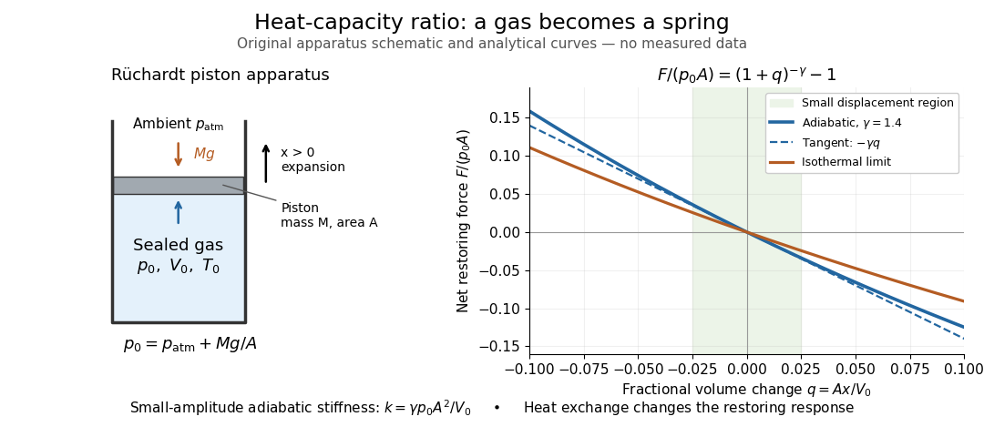
The Rüchardt experiment infers heat capacity ratio from the period of an oscillation of a piston supported by trapped gas. Use a vertical precision cylinder with a close-fitting movable piston, known moving mass $M$, face area $A$, trapped equilibrium volume $V_0$, and local atmospheric pressure $p_{\mathrm{atm}}$. With negligible static friction, force balance gives the absolute gas pressure $p_0=p_{\mathrm{atm}}+Mg/A$, where $g$ is gravitational acceleration. Displace the piston slightly and release it: compression raises pressure, and expansion lowers it, producing a restoring force. The oscillation is a mechanical probe of thermal response, without separately measuring two heat inputs. ^[ref]

Let $x$ be upward displacement from equilibrium, so $V=V_0+Ax$. For constant heat capacity ratio and a reversible adiabatic process, the net upward force, including the ambient load and weight, isThe linear approximation requires $|Ax|/V_0\ll 1$. Applying Newton's second law gives simple harmonic motion withHere ${\omega }_0$ is the undamped angular frequency and $\mathcal{T}$ the undamped oscillation period, rather than temperature. Record repeated cycles, measure $M,A,V_0,p_{\mathrm{atm}}$ independently, and include all connected trapped volume. An illustrative model with $M=0.020\mathrm{kg}$, $A=2.0\times 10^{-4}{\mathrm{m}}^2$, $V_0=0.010{\mathrm{m}}^3$, $p_{\mathrm{atm}}=100000\mathrm{Pa}$, $g=9.81\mathrm{m}{\mathrm{s}}^{-2}$ and $\gamma =1.4$ gives $p_0=100981\mathrm{Pa}$ and $\mathcal{T}\simeq 1.182\mathrm{s}$. These stipulated values are not measurements.

In Shearwood and Sloan's implementation, piston-mounted magnets induce an electromotive force in a stationary coil through Faraday's law of induction; an oscilloscope records the signal. They observed faster oscillations at smaller trapped volume values and stronger damping at small cylinder volume values. The signal tracks velocity locally, so its amplitude is not directly piston displacement. Calibration also identified inlet dead space beyond the graduated cylinder volume. ^[ref]

Repeat at smaller initial amplitudes to test the linear approximation, and compare several $V_0$ values. Heat transfer weakens the restoring force toward the isothermal process limit, biasing the inference toward $1$. Check leakage through resting-piston drift and before-and-after trapped volume readings. For viscous damping with envelope $e^{-t/\tau }$, the measured angular frequency obeys ${\omega }_0^2={\omega }_d^2+{\tau }^{-2}$; this correction does not remove thermal leakage. Internal equilibration must be faster than an oscillation period, with heat transfer and leakage slow over a run. Large amplitude or sticking friction require a richer model. ^[ref]

A heating curve records temperature against accumulated supplied heat under a specified constraint. Within one thermodynamic phase, its slope is $dT/dQ=1/C_X$, where $C_X$ is the constrained heat capacity. A latent heat plateau instead records changing phase fraction at the phase coexistence temperature. The sensible heat example combines two sloping intervals and a melting plateau in one heating budget.

Molar heat capacity is heat capacity divided by amount of substance $n$, with units $\mathrm{J}\mathrm{mo}{\mathrm{l}}^{-1}{\mathrm{K}}^{-1}$. Its constraint must still be specified: $C_{V,\mathrm{m}}=C_V/n$ and $C_{p,\mathrm{m}}=C_p/n$. For the classical monatomic gas example in heat capacity, these are $3R/2$ and $5R/2$, where $R$ is the molar gas constant. Some textbooks use $C_V$ and $C_p$ for these per-mole quantities; the convention here reserves them for the whole sample.

Upper records of iid observations with a continuous distribution have transition density $f(w)/(1-F(v))$ above the latest record $v$. Consequently the cumulative hazard $\Lambda (v)=-\log (1-F(v))$ transforms consecutive record increments into independent unit exponentials. Record counts below a level $t$ with $F(t)<1$ are therefore Poisson with mean $\Lambda (t)$. Set the count to zero if the first record exceeds the level. At a finite upper endpoint with $F(t)=1$, the count is infinite instead of a finite-mean Poisson variable.

These are the optimal volume-fraction bounds for three-dimensional statistically isotropic two-phase conductivity with $0<a_1<a_2$. Constant phase polarization trial fields reduce the variational principle to a scalar quadratic optimization. The upper trial functional is minimized; the lower one is maximized.

For uniformly distributed rotations of a two-dimensional conductivity tensor with positive principal values $a\le b$, the Hashin-Shtrikman conductivity variational principle with isotropic comparison $cI$ yields $H(c)I$. Averaging a rotated diagonal tensor replaces it by half its trace times the identity. Since $H^{\prime }(c)=(a-b{)}^2/(a+b+2c{)}^2$, the admissible comparison endpoints give $a(a+3b)/(3a+b)\le C_{\mathrm{eff}}\le b(3a+b)/(a+3b)$ within the statistically isotropic polycrystal model.

For infinite sets in ZFC, the Hartogs number is the successor of the input cardinal. Every smaller ordinal injects into the input, whereas that successor does not. An infinite successor cardinal ${\kappa }^{+}$ is regular: a cofinal family of at most $\kappa$ ordinals below it would have union of cardinal at most $\kappa \cdot \kappa =\kappa$, a contradiction. Finite inputs give finite successor cardinals, so the formulation in terms of alephs requires an infinite input. The general Hartogs theorem itself does not require choice.

For the growing matter-era spectrum $P(k,\tau )=Ak(\tau /{\tau }_{\mathrm{eq}}{)}^4$ and Gaussian Fourier window $W(kr)=e^{-(kr{)}^2/2}$, integration gives the displayed smoothed matter density variance. A physical Hubble-radius window has $r=1/(aH)=\tau /2$, making its variance independent of crossing time. The dimensionless mode variance $k^{3}P/(2{\pi }^2)$ is likewise constant at $k\tau =2$. A pure $P\propto k$ spectrum needs ultraviolet-convergent smoothing: a real-space top-hat alone leaves a logarithmic divergence.

// Target: cosmology.bigb

The Poisson kernel for the upper half-space gives an isometric bijection from finite real or complex Borel measures, with their total variation norm of a measure, onto the harmonic Hardy space of the upper half-space. The kernel has unit mass, so Tonelli theorem gives the upper norm bound. Its approximate identity property gives weak-star convergence to the original measure and hence the reverse norm bound. For surjectivity, the mean value property for harmonic functions bounds each shifted harmonic function; bounded harmonic uniqueness gives $u(\cdot ,s+t)=P_t\ast u(\cdot ,s)$. A weak-star limit of the uniformly bounded measures $u(\cdot ,s)dx$ then gives the required boundary measure. In particular $|u(x,t)|\le c_d{t}^{-d}\Vert u{\Vert }_{h^1}$, where $c_d=\Gamma ((d+1)/2)/{\pi }^{(d+1)/2}$.

On a connected compact oriented Riemannian manifold without boundary, a top-degree form is $f{\mathrm{vol}}_g$. Its exterior derivative is automatically zero, and the Hodge codifferential vanishes exactly when $df=0$. Thus it is harmonic exactly when $f$ is constant. Equivalently the Hodge star operator identifies this space with harmonic functions. Without connectedness the dimension is the number of connected components.

On a domain carrying a branch of the complex logarithm, the holomorphic function $-i\mathrm{Log}z$ has real part equal to the chosen angle and imaginary part $-\log |z|$. These are harmonic conjugates; their level sets are rays and circles, meeting orthogonally. For the principal real arctangent $\varphi =\arctan (y/x)$, its domain has the two components $x>0$ and $x<0$. The corresponding holomorphic functions are $-i\mathrm{Log}z$ and $-i\mathrm{Log}(-z)$, using the complex logarithm on the right half-plane. This formulation does not assert a globally single-valued angle on the punctured plane.