Let commuting elements $a,b$ have finite coprime orders $m,n$. Their cyclic subgroups have trivial intersection by Lagrange's theorem. If $(ab{)}^k=1$, then $a^k=b^{-k}$ belongs to this intersection, so $m\mid k$ and $n\mid k$. Thus $mn\mid k$. Conversely, $(ab{)}^{mn}=1$ because the elements commute. This proves the displayed order formula.

Over a cone point of order $m$, a cycle of length $\ell$ in the monodromy on sheets has ramification degree $\ell$ and residual cone angle $2\pi \ell /m$. The lifted inherited hyperbolic metric is smooth precisely when every such cycle has length $m$. Equivalently the subgroup defining the cover meets no conjugate of a nonidentity power of a cone generator.

Pair the $2s$ edges of an oriented hyperbolic polygon by length-preserving identifications reversing their boundary directions. Label the pairs by generating elements $A_1,\dots ,A_s$ of a finite group $T$. Glue the corresponding edge of a copy labelled $g$ to its mate in the copy labelled $g{A}_k$. Left multiplication of labels defines the $T$ action. A vertex cycle of a paired polygon has angle sum ${\theta }_j$ and accumulated gluing word $C_j\in T$ of order $q_j$; above it lie $|T|/q_j$ vertices, each of cone angle $q_j{\theta }_j$. The action is free away from vertices, and the vertex stabilizers are conjugates of $⟨C_j⟩$. If the base cone has integer order $m_j=2\pi /{\theta }_j$ and $q_j\mid m_j$, this is an orbifold covering, with lifted cone order $m_j/q_j$. The lift is smooth exactly when $q_j=m_j$.

An $n$-sheeted surface cover of an orbifold of underlying genus $g_0$ with $r$ cone points has the displayed ordinary Euler characteristic, where $c_i$ is the number of cycles of the $i$th cone monodromy permutation. The ramification deficit over that point is $n-c_i$, so the formula follows by counting lifted vertices, edges and faces, or by the Riemann-Hurwitz formula. If every cone cycle has its full prescribed length, this equals $n{\chi }_{\mathrm{orb}}$.

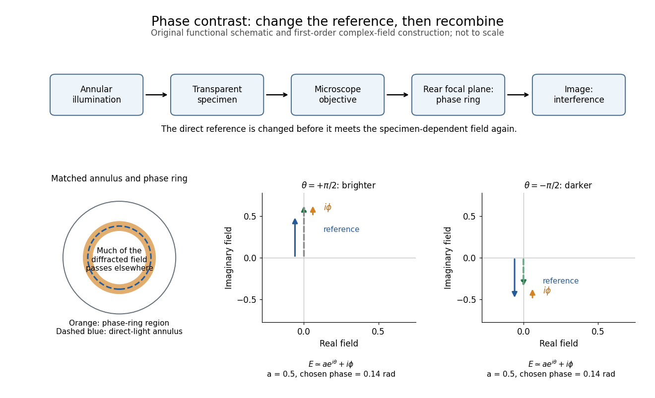
Phase-contrast microscopy converts specimen-dependent phase differences into visible light intensity differences. It can reveal structures in living, unstained biological cells, allowing their changes to be followed without first making an absorbing preparation.^[ref] The key question is how an optical microscope can read a phase when an ordinary detector records light intensity.

Consider a transparent specimen with complex amplitude transmission $t(x,y)=e^{i\varphi (x,y)}$. In ideal in-focus coherent imaging with all relevant spatial frequencies transmitted, its image has $I=|t{|}^2=1$: varying $\varphi$ alone produces no brightness detail. This is a particular model, not a claim that all transparent specimens are invisible. Diffraction, defocus, absorption and a finite optical pupil can already change a real image.

A phase-contrast microscope images an illuminating annulus onto a phase plate ring near the objective's rear focal plane. The aligned ring attenuates and shifts direct light relative to most diffracted light; their interference changes image brightness.^[ref]

The method is beautiful because the bright direct beam becomes its own reference: a small specimen-dependent complex amplitude can interfere with it and change the image at first order. Merely magnifying an invisible phase pattern would leave $|t{|}^2$ unchanged.

In a simple two-mirror oscillator, laser threshold is the small-signal optical gain at which a resonant optical normal mode exactly replaces its round-trip intensity loss. Assume constant intensity coefficients $g$ and $\alpha$ throughout a one-way distance $L$, and mirror intensity reflectivities $0<R_1,R_2\le 1$. One round trip has multiplierTwo traversals give the distance $2L$; multiplying the two mirror factors completes the bookkeeping. Setting $M=1$ and taking a logarithm givesThe reflectivities here are intensity fractions, not field-amplitude reflectivities. A shorter gain region or nonuniform loss requires replacing the path exponent by the appropriate path integral. The balance also presumes a permitted resonant optical normal mode. ^[ref].

For $L=0.50\mathrm{m}$, $R_1=1$, $R_2=0.90$ and $\alpha =0.10{\mathrm{m}}^{-1}$, the threshold is $g_{\mathrm{th}}\approx 0.2053605{\mathrm{m}}^{-1}$. At $g=0.15{\mathrm{m}}^{-1}$, $M\approx 0.946144$: a small circulating signal decays even though the material has positive optical gain. At $g=0.30{\mathrm{m}}^{-1}$, $M\approx 1.099262$: the signal initially grows. Raising passive loss or lowering mirror reflectivity raises laser threshold.

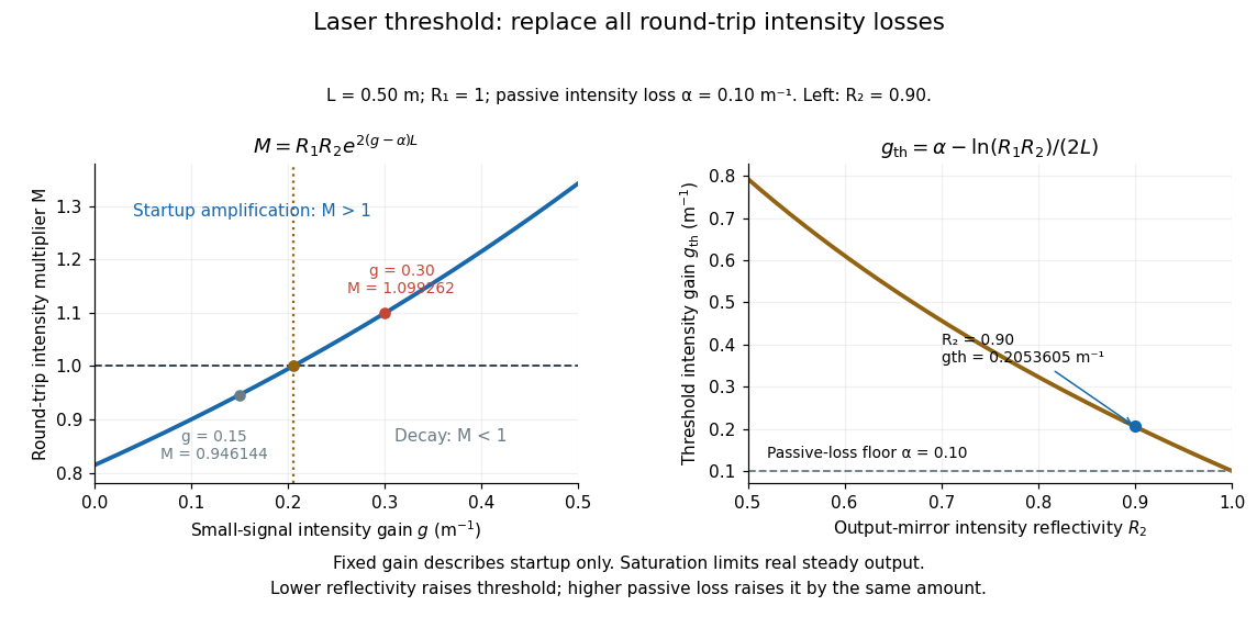
For $M>1$, the fixed-gain recurrence predicts startup amplification, not infinite actual output. Growing light intensity depletes the available population inversion, reducing optical gain through saturation. In the simplest steady oscillator, the saturated round-trip gain balances loss and pumping supplies the outgoing power and dissipated energy. The small-signal model locates the onset; it does not determine the final output power. ^[ref].

Consider one selected polarization of waves, represented by complex fields $E_1(t)$ and $E_2(t)$ at two sampling positions. Suppose their second moments are finite and stationary: $J_j=⟨|E_j(t){|}^2⟩$ and the following uncentered wave-field correlation do not depend on the absolute time $t$. DefineThe star denotes the complex conjugate; brackets denote an ensemble average. A long detector average estimates this quantity only if it adequately samples the fluctuations. The superscript $1$ identifies a field correlation: it does not mean the autocorrelation of the measured light intensity. The one-position version is $g^{(1)}(\tau )=⟨E^{\ast }(t)E(t+\tau )⟩/⟨|E{|}^2⟩$, so $g^{(1)}(0)=1$ for every nonzero field covered by this definition; this alone says nothing about its correlation at nonzero delay. ^[ref].

The Cauchy-Schwarz inequality gives $0\le |g_{12}^{(1)}(\tau )|\le 1$. At a specified delay, magnitude one means $E_2(t+\tau )=a{E}_1(t)$ in mean square for a fixed nonzero complex $a$: the samples have a reproducible relation in both wave amplitude and wave phase. Magnitude zero means the averaged field cross term vanishes. It need not mean statistical independence. A deterministic phase difference changes the argument of $g^{(1)}$, not its complex modulus; a distorted but fixed wavefront can therefore remain fully coherent. ^[ref].

To see the observable, recombine the samples in the same detected spatial mode with matched wave polarizations. With a common positive conversion factor $C$, let $I_j=C{J}_j$ be the single-arm light intensities reaching that detector. Adding $E_1(t)+e^{i\varphi }{E}_2(t+\tau )$ givesThis follows simply by expanding the squared complex modulus and averaging, then taking the maximum and minimum as $\varphi$ spans a full cycle. The extra wave phase scan must leave $I_1,I_2$ and the magnitude of the correlation effectively unchanged. Thus interferometric visibility equals $|g^{(1)}|$ only for equal nonzero light intensities and ideal mode matching. For $I_2/I_1=1/4$, perfectly coherent beams have interferometric visibility $0.8$; a measured value $0.4$ would imply $|g^{(1)}|=0.5$ under these assumptions. Orthogonal linear polarizations, background light, unresolved interference fringes or vibrations can reduce measured contrast further. One absent arm gives zero contrast and makes the normalized two-sample correlation undefined.

At the boundary of an Oppenheimer-Snyder cloud, its areal radius is $R=a\sin {\chi }_0$. Matching to a Schwarzschild metric gives $M=4\pi \rho R^3/3=a_{\max }{\sin }^3{\chi }_0/2$. Thus ${\sin }^2{\chi }_0=2M/R_0$ and $a_{\max }=\sqrt{R_0^3/(2M)}$. The boundary is a radial timelike geodesic with specific Killing energy $\sqrt{1-2M/R_0}=\cos {\chi }_0$. Its radial equation is ${\dot{R}}^2=2M/R-2M/R_0$. The induced metric and the angular extrinsic curvature agree on both sides, so no surface layer is required.

A boundary clock in Oppenheimer-Snyder collapse reads $\tau =a_{\max }(\eta +\sin \eta )/2$. Its event horizon crossing occurs at $R=2M$, giving the displayed angle, and the final curvature singularity occurs at $\eta =\pi$. The remaining proper time is $a_{\max }(\pi -{\eta }_H-\sin {\eta }_H)/2$. For $R_0\gg 2M$ this approaches $4M/3$, but it is not exactly that value for finite release radius.

Radial outgoing null geodesics in the interior of Oppenheimer-Snyder collapse obey $d\chi /d\eta =1$. Trace the ray crossing the boundary at $({\eta }_H,{\chi }_0)$ backward: it starts at the centre at $\eta ={\eta }_H-{\chi }_0$. This ray is the event horizon; it can exist inside the cloud before the surface crosses $R=2M$. An event horizon is determined by global escape to future null infinity, rather than by a local stopwatch signal.

The comoving dust ball $0\le \chi \le {\chi }_0<\pi /2$ in the Oppenheimer-Snyder model is an Oppenheimer-Snyder cloud. Its pressureless matter has uniform density on each constant-proper time slice and reaches a simultaneous final singularity in the ideal homogeneous model.

The syntactic grouping convention for successive operators of the same precedence. Left grouping of subtraction makes a-b-c mean (a-b)-c; it does not make subtraction an associative operation.

A unital star-subalgebra of the bounded operators on a Hilbert space that is closed in the weak operator topology, equivalently in the strong operator topology. The Von Neumann double commutant theorem makes these conditions equivalent to equality with the double commutant of an operator algebra. It is norm closed and hence a C-star algebra.

A vector is cyclic for an operator algebra when its orbit under that algebra has dense linear span. This is distinct from requiring the powers of one chosen operator to span the space. If the algebra is linear, its orbit itself is already a vector subspace.

For a lattice system, finite-region observable algebras ${\mathcal{A}}_{\Lambda }$ embed into larger ones by tensoring with the identity. Their union has a norm closure called the quasi-local observable algebra, a C-star algebra. It describes finite-support observables and norm limits of such observables. An operator flipping every spin of an infinite lattice need not belong to it: successive finite-region flips are not norm-Cauchy. Restrictions to this algebra can therefore lose relative-phase information retained by increasingly nonlocal finite-system observables.

A commuting diagonal expectation value has one transverse eigenvalue vector for each brane. In the covariant derivative normalization $D_a\varphi ={\partial }_a\varphi +i[A_a,\varphi ]$, the off-diagonal gauge field has mass $m^2={\sum }_I({\varphi }_1^I-{\varphi }_2^I{)}^2$. The corresponding stretched string has mass $|X_1-X_2|/(2\pi {\alpha }^{\prime })$ in its massless oscillator sector. Equality fixes the displayed scalar-position normalization, up to a common coordinate origin. The trace describes center-of-mass motion and the eigenvalue difference describes separation.

For two static parallel D-branes separated transversely by $d$, the open bosonic string mass spectrum becomes $M^2=d^2/(4{\pi }^2{\alpha }^{\prime 2})+(N-1)/{\alpha }^{\prime }$. The classical stretching contribution is the square of the string tension times the separation, while the oscillator vacuum contributes the intercept term. Thus the ground state is a tachyon for $d<2\pi \sqrt{{\alpha }^{\prime }}$, massless at equality, and massive above it. Its real rest energy, when stable, is $\sqrt{d^2/(4{\pi }^2{\alpha }^{\prime 2})-1/{\alpha }^{\prime }}$; the vacuum correction belongs to energy squared and is not an additive fixed subtraction from the stretching energy. Angled branes change oscillator moding and require a different formula.

For an ordinary critical open string with all Neumann boundary conditions, there are 24 independent transverse creation oscillators at each positive mode number $n$. Summing their nonnegative occupation numbers gives one factor $(1-w^n{)}^{-24}$. The coefficient $d_p=[w^p]F(w)$ counts oscillator polarizations at level $p$, excluding continuous center-of-mass momentum and additional endpoint multiplicities. Cauchy coefficient formula gives $d_p=(2\pi i{)}^{-1}\oint F(w)w^{-p-1}dw$.

An annulus is the region between two concentric circles.

A neighbourhood of a point is a set containing an open set that contains that point.