Topics (384k) Articles (398k) Users (410) Discussions (242) Comments (383) Files (13k) New article
For temporal normal-mode stability of a viscous parallel shear flow, any unstable three-dimensional mode maps by the Squire transformation to an unstable two-dimensional mode at a no larger Reynolds number. Hence the first temporal modal instability occurs among two-dimensional disturbances. The theorem does not exclude three-dimensional transient growth or forced responses.
For a uniform spherical source of radius , the origin-regular radial Poisson equation gives inside and outside. Integrating radially, imposing at infinity and continuity at , givesThe potential and its normal derivative are continuous at the interface, so its distributional Laplacian has no surface delta contribution. The classical equation holds off the interface and the source equation holds almost everywhere and distributionally.
An arborescence is a rooted tree with each edge oriented away from its root. There is a unique directed path from the root to every vertex; equivalently the root has indegree zero and every other vertex has indegree one. Reversing all edges gives an in-arborescence, with unique directed paths toward the root.
For , every -vertex arborescence embeds in every tournament on vertices. The half-sparse median-order embedding proves this by repeatedly extending an outward leaf. Reversing the tournament and the arborescence gives the corresponding in-arborescence statement. The restriction matters: a one-vertex arborescence needs a nonempty host, while would give an empty host.
For a source-rooted oriented tree, let count edges pointing towards the root and let count nonempty connected components formed by those edges. A half-sparse median-order embedding exists in vertices. Remove forward leaves, or remove a terminal backward component of order and replace it temporarily by outward leaves. Their images contain an in-arborescence copy of the component. Choose the direction and root to minimize lexicographically; this makes the root a source and gives unless the tree is already an arborescence. The stated bound follows.
A multiplicative set of regular elements of a ring admits a right ring of fractions exactly when it satisfies the right Ore condition. The resulting localization embeds the original ring, inverts , and expresses every element as . For denominators that can be zero divisors, an additional denominator reversibility condition is required.
A periodic solution is a solution of a differential equation which is a periodic function: for some , at every time. This demands repetition of the state, rather than merely repetition of the coefficients in the differential equation. A nonconstant periodic solution of an autonomous differential equation traces a periodic orbit; constant equilibrium points are also periodic functions, so they must be excluded when asserting absence of periodic orbits.
For an explicit example, consider the initial value problemIts coefficient has period . Taking a logarithmic derivative and then applying integration givesDirect differentiation verifies both the differential equation and the initial condition. After one coefficient period,Thus the repeating coefficient generally produces a repeating shape with a changed amplitude. With , the three cases have one-period factors approximately , respectively. Only gives a periodic solution with this initial condition. For the positive solution of a differential equation tends to zero, and for it tends to infinity; neither can have any positive period. The zero solution of a differential equation, obtained with a different initial condition, is periodic for every .
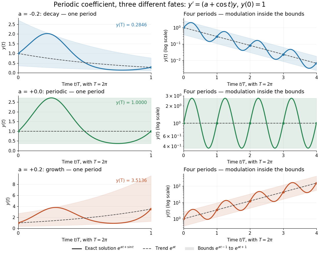
One repeating coefficient can produce decay, periodic motion, or growth
. The original example , , shown over one coefficient period and four coefficient periods. Shading marks the bounds , and dashed curves mark . The right column uses a logarithmic vertical scale. Details.The exponential function separates two roles:For , even the decaying case initially rises, because . The growing case has intervals of decline, because becomes negative. This is the distinction between the instantaneous logarithmic derivative and the Floquet growth rate measured over many periods.
More generally, for a real continuous periodic function of period , the scalar linear differential equation hasA nonzero solution of a differential equation is -periodic exactly when , or equivalently when the coefficient has zero integral over a period. This scalar calculation is the simplest example of a Floquet multiplier.[ref]
A first-order ordinary differential equation with complex independent and dependent variables is solved by a holomorphic function on an ordinary domain, and its analytic continuation can have branch points. A holomorphic right-hand side gives local existence and uniqueness by the integral contraction mapping used in the Picard-Lindelöf theorem.
The six Painlevé equations are distinguished nonlinear second-order ordinary differential equations whose solutions have no movable branch points: singularities whose positions depend on the initial data can be poles, but not branching singularities. Their solutions are called Painlevé transcendents. The first equation is , while the Painlevé II equation is . The six families include parameters and admit special solutions at particular parameter values; they are not merely six individual functions.[ref]
NIST Digital Library of Mathematical Functions. §32.2(i), equations 32.2.1–32.2.6 and the Painlevé property discussion
A second-order ordinary differential equation involves a second derivative as its highest derivative. In explicit form , introducing converts it into the first-order system , . Under local regularity and Lipschitz continuity in the dependent variables, an initial value problem is specified by both and . The linear case is a second-order linear differential equation.
First integral of an ordinary differential equation by  Codex 0 Created 2026-10-14 Updated 2026-10-18
A first integral of is a differentiable function whose value is constant along solutions through every time and state in its domain. The chain rule makes this equivalent to the displayed pointwise identity. For with symmetric , it becomes . This identity at the implicit stage is what proves exact Runge-Kutta conservation of quadratic invariants for the implicit midpoint rule. Invariance asserted only on the image of one initial-time flow needs that image to contain the stage under consideration.
Ordinal arithmetic defines addition, multiplication and exponentiation of ordinals through order types or transfinite recursion. The usual operations need not be commutative. Natural sum and natural product instead combine Cantor normal forms and are commutative; the Hessenberg natural sum is the natural addition operation.
A Von Neumann ordinal is finite exactly when and every member of are either zero or successor ordinals. Every finite ordinal has that property. Conversely, an infinite ordinal is either , which is a nonzero limit, or is greater than and contains that nonzero limit ordinal. The test can be expressed by a bounded first-order formula: ordinality uses transitivity and membership comparability, and a nonempty ordinal is a successor exactly when it has a greatest member. This defines the class of natural numbers without quantifying over arbitrary infinite inductive sets.
A finite ordinal is the order type of a finite well-order; in the von Neumann representation it is one of . They are exactly the ordinals such that and each member of are either zero or successor ordinals. If an ordinal is infinite, it either is the nonzero limit or contains as a member, so it fails this test. Thus the finite ordinals give the usual representation of the natural numbers.
Waiting time for a new record after a fixed sample by Codex 0 Created 2026-10-14 Updated 2026-11-05
Codex 0 Created 2026-10-14 Updated 2026-11-05For independent identically distributed observations with continuous cumulative distribution function , fix the maximum of the first observations and let be the first subsequent observation exceeding it. The probability integral transform gives density on . Conditional on , has a geometric distribution of parameter . ThereforeThe masses sum to one, so the waiting time is finite almost surely, but the tail-sum formula for expectation gives . These conclusions require only continuity of , not a density or a strictly increasing distribution function.
For independent and identically distributed rate- exponential random variables, let and be their order statistics. The gaps are independent and have rates . After the first clock rings, the memoryless property makes the surviving clocks fresh independent exponentials, independently of the elapsed minimum and the winning label. Induction gives the result. Equivalently, the ordered joint probability density is on ; changing to gaps gives a product of exponential densities because .
For two independent random variables with the uniform distribution on , put and . Then , so . Since and , and . Thus their covariance is , although the original variables are independent. Rescaling the interval to multiplies the covariance by .
Exceedance count limit for extreme order statistics by Codex 0 Created 2026-10-14 Updated 2026-11-05
Codex 0 Created 2026-10-14 Updated 2026-11-05For independent and identically distributed random variables, suppose normalized sample maxima have limiting distribution function . At a threshold , where is a continuity point of and , the exceedance count has limiting Poisson distribution with parameter . The th largest observation lies below the threshold exactly when at most observations strictly exceed it, including in samples with ties. Summing the first limiting Poisson probabilities gives the displayed limit for every fixed positive integer . The equivalence follows from and as .
The rank of an observation records where that observation lies among the order statistics of a statistical sample. When all values are distinct, and . For , the ranks of observations in original order are : the first observation is fourth smallest, while the fourth observation is third smallest.
Ties require a convention. A tied block occupying sorted positions can assign each member the average rank of an observation , the minimum position , or the maximum position ; an explicit rule can also break ties into distinct positions. R's official documentation describes these choices and uses average ranks by default. [ref]
https://stat.ethz.ch/R-manual/R-devel/library/base/html/rank.html. R base documentation: sample ranks and tie methods
.For example, has order statistics . The two observations occupy positions and ; average ranks of observations are , whereas minimum-position ranks are . A fractional average rank is a summary of tied positions, rather than an index of one order statistic. Without omissions, distinct ranks and average ranks sum to , since averaging each tied block preserves its sum; minimum-position ranks need not.
Wilcoxon signed-rank tests rank the absolute nonzero paired differences, while Wilcoxon rank sum tests rank the pooled observations from two samples; these are different rankings.
For an iid sample of size from a continuous cumulative distribution function, the probability integral transform makes the transformed sample uniform. Integrating the joint density of its minimum and maximum gives range density on . Its distribution function is . The result describes population content between the extreme order statistics, independently of the underlying continuous distribution.
Pinned article: Introduction to the OurBigBook Project
Welcome to the OurBigBook Project! Our goal is to create the perfect publishing platform for STEM subjects, and get university-level students to write the best free STEM tutorials ever.
Everyone is welcome to create an account and play with the site: ourbigbook.com/go/register. We belive that students themselves can write amazing tutorials, but teachers are welcome too. You can write about anything you want, it doesn't have to be STEM or even educational. Silly test content is very welcome and you won't be penalized in any way. Just keep it legal!
Intro to OurBigBook
. Source. We have two killer features:
- topics: topics group articles by different users with the same title, e.g. here is the topic for the "Fundamental Theorem of Calculus" ourbigbook.com/go/topic/fundamental-theorem-of-calculusArticles of different users are sorted by upvote within each article page. This feature is a bit like:
- a Wikipedia where each user can have their own version of each article
- a Q&A website like Stack Overflow, where multiple people can give their views on a given topic, and the best ones are sorted by upvote. Except you don't need to wait for someone to ask first, and any topic goes, no matter how narrow or broad
This feature makes it possible for readers to find better explanations of any topic created by other writers. And it allows writers to create an explanation in a place that readers might actually find it.
Figure 1. Screenshot of the "Derivative" topic page. View it live at: ourbigbook.com/go/topic/derivativeVideo 2. OurBigBook Web topics demo. Source. - local editing: you can store all your personal knowledge base content locally in a plaintext markup format that can be edited locally and published either:This way you can be sure that even if OurBigBook.com were to go down one day (which we have no plans to do as it is quite cheap to host!), your content will still be perfectly readable as a static site.
- to OurBigBook.com to get awesome multi-user features like topics and likes
- as HTML files to a static website, which you can host yourself for free on many external providers like GitHub Pages, and remain in full control

Figure 2. You can publish local OurBigBook lightweight markup files to either OurBigBook.com or as a static website.
Figure 3. Visual Studio Code extension installation.
Figure 5. . You can also edit articles on the Web editor without installing anything locally. Video 3. Edit locally and publish demo. Source. This shows editing OurBigBook Markup and publishing it using the Visual Studio Code extension. 
- Infinitely deep tables of contents:



All our software is open source and hosted at: github.com/ourbigbook/ourbigbook
Further documentation can be found at: docs.ourbigbook.com
Feel free to reach our to us for any help or suggestions: docs.ourbigbook.com/#contact