Topics (384k) Articles (398k) Users (410) Discussions (242) Comments (383) Files (13k) New article

A physics educator and coauthor of College Physics by Paul Peter Urone and others. The textbook uses a consistent problem-solving approach that connects a physical situation with an equation and a reasoned check of the answer. Everyday and biomedical examples let students apply the same mechanics, thermodynamics and electromagnetism to practical questions rather than treating each equation as an isolated rule.[ref]
College Physics by Paul Peter Urone and others. Preface: senior contributing authors, applications and problem-solving approach
A physicist whose research includes the acoustics of musical instruments and the human voice, and whose teaching materials connect wave models with accessible experiments.[ref]
Joe Wolfe: educational videos and pages by Joe Wolfe. Introduction: musical-instrument and voice acoustics; Physclips teaching resources
For example, his sound-wave experiment moves a microphone along a tube to locate standing wave pressure minima and maxima. Comparing these positions with the tube boundaries helps distinguish pressure nodes from displacement nodes, turning an otherwise easy-to-confuse distinction into a direct measurement.[ref]Interesting and inexpensive experiments for high school physics by Joe Wolfe. Printed pp. 10–11: microphone measurements of standing waves and distinction between pressure and displacement
An astronomer and historian who reconstructed the quantitative reasoning behind early celestial mechanics. His analysis of Johannes Kepler’s difficulty predicting the position of Mars shows why the observer’s own orbit matters: correcting the model of Earth’s motion changes the inferred position of another planet. Repeated observations separated by a Martian year allowed Kepler to compare Earth’s position from different viewing directions, exposing an error in the assumed terrestrial orbital eccentricity.[ref]
The great Martian catastrophe and how Kepler fixed it by Owen Gingerich. Printed pp. 52–53 and Fig. 4: Earth-orbit correction and observations separated by 687 days
Coauthored the helium Hanbury Brown and Twiss effect comparison, isolating the effect of quantum statistics through matched-temperature boson and fermion measurements with negligible interactions.[ref]
Coauthored the helium correlation experiment in which a defocusing laser lens deepened the observed fermion antibunching signal by reducing resolution-induced averaging.[ref]
Coauthored the Hanbury Brown and Twiss effect study comparing helium-3 and helium-4 correlation lengths; the measured ratio agreed with the expected inverse-mass ratio.[ref]
Coauthored the helium Hanbury Brown and Twiss effect comparison, reconstructing spatial correlation functions from individual atoms’ arrival positions and times after release.[ref]
Coauthored a Hanbury Brown and Twiss effect comparison showing opposite helium-4 boson and helium-3 fermion correlations in one apparatus.[ref]
An atomic-physics researcher whose joint study used excited helium atoms to detect the Hanbury Brown and Twiss effect. Measuring pair arrivals converts otherwise invisible many-particle interference into a statistical pattern, linking detection probabilities with the distinction between Bose-Einstein statistics and Fermi-Dirac statistics.[ref]
Comparison of the Hanbury Brown-Twiss effect for bosons and fermions by T. Jeltes and others. Abstract and pp. 2–4: metastable-atom detection and exchange interference
A researcher whose team compared bosons and fermions using nearly identical trapped-cloud conditions. The contrasting pair correlations of helium-4 and helium-3 therefore isolated exchange statistics rather than ordinary attractive or repulsive forces between particles.[ref]
Comparison of the Hanbury Brown-Twiss effect for bosons and fermions by T. Jeltes and others. Abstract and pp. 3–4: matched trapping conditions and negligible interactions
A researcher whose joint experiment measured fermionic atom antibunching. Atoms released from a trap struck a detector that recorded position and arrival time. Their pair distribution showed fewer nearby detections than statistically independent arrivals would produce, a signature of Fermi-Dirac statistics.[ref]
Comparison of the Hanbury Brown-Twiss effect for bosons and fermions by T. Jeltes and others. pp. 3–4 and Fig. 2: detector events and normalized pair probability
An experimental researcher whose team compared the Hanbury Brown and Twiss effect in two helium isotopes. Detecting individual released atoms revealed enhanced close pairs for bosons and suppressed pairs for fermions, making their different exchange statistics directly observable.[ref]
Comparison of the Hanbury Brown-Twiss effect for bosons and fermions by T. Jeltes and others. Abstract, pp. 3–4 and Fig. 2: isotope comparison and pair correlations
Wolfgang Pauli introduced the Pauli exclusion principle to explain the organization of electron configurations and the closing of electron shells. In its later wave function formulation, exchanging two identical fermions reverses the sign of the joint quantum state. Putting both fermions in the same one-particle quantum state would leave the product unchanged, so antisymmetrizing gives zero. For electrons, a spatial orbital can still contain two occupants with opposite spin, because their full one-particle quantum states differ.[ref]
Exclusion principle and quantum mechanics by Wolfgang Pauli. Nobel lecture, discussion of closed shells and antisymmetric functions, printed p. 31

Portrait of Wolfgang Pauli
. Bettina Katzenstein / ETH Zürich; ETH-Bibliothek Zürich, Bildarchiv, Portr 01042. Creative Commons Attribution-ShareAlike 3.0 Unported, via Wikimedia Commons. Source.A researcher in optical metrology who compared two NIST cryogenic radiometers using common photodiode trap detectors. Each radiometer independently calibrated the detectors’ spectral responsivity, allowing consistency to be tested without assuming that either instrument was error-free. The comparison illustrates electrical substitution radiometry: absorbed optical power is related to the electrical heating needed to produce the same thermal response.[ref]
Comparison of Two Cryogenic Radiometers at NIST by Jeanne M. Houston and others. Abstract and §§2–5: trap-detector transfer, substitution protocols and uncertainty comparison
A researcher in optical measurement whose work with Jeanne M. Houston establishes detector spectral responsivity. A detector’s electrical signal is compared with a calibrated reference while the illumination wavelength is varied; subtracting dark current and monitoring source changes separates optical response from instrumental offsets. The resulting calibration converts a measured current into optical power, with an explicit dependence on wavelength rather than a single sensitivity number.[ref]
Spectroradiometric Detector Measurements: Ultraviolet, Visible, and Near-Infrared Detectors for Spectral Power by Thomas C. Larason and others. §§3.2, 4.2 and 7.2: detector-comparison apparatus, spectral readout and measurement controls
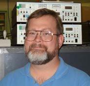
Portrait of Thomas C. Larason
. Source. Yoshihiro Ohno develops the physical interpretation of optical measurements used in vision. His account distinguishes radiometry, which measures optical radiation, from photometry, which weights visible radiation by the eye's spectral response. Equal optical powers at different wavelengths therefore need not have equal luminous output. A photometer can implement that weighting through its spectral sensitivity, or a spectrally resolved measurement can be weighted afterward. This connects a reported brightness-related quantity with its detector and wavelength conventions.[ref]
Radiometry and Photometry: Review for Vision Optics. 2000 chapter, abstract: radiometric/photometric quantities and spectral weighting
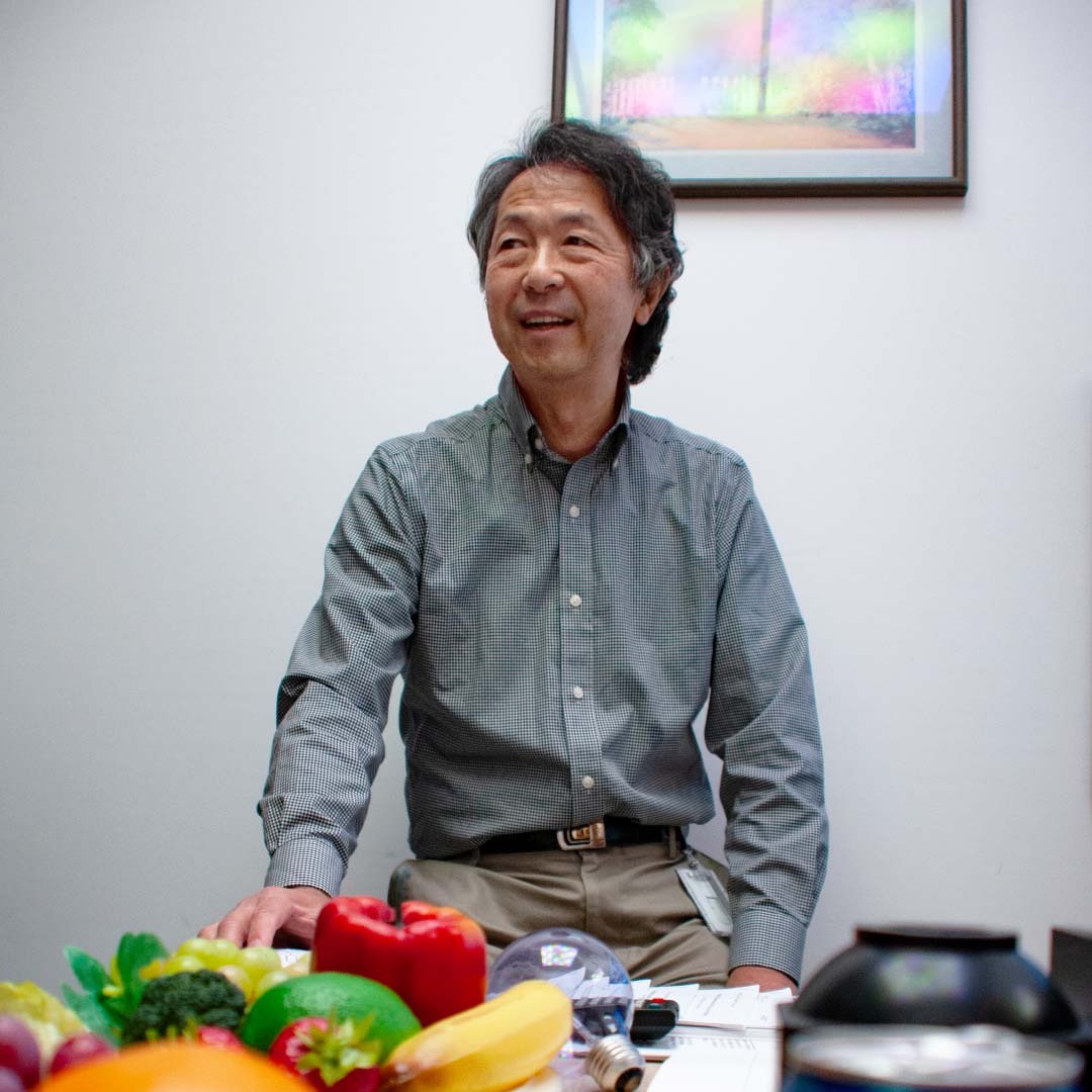
Portrait of Yoshihiro Ohno
. Yoshihiro (Yoshi) Ohno in NIST’s Spectrally Tunable Lighting Facility. Credit: R. Wilson/NIST. No reuse licence is asserted. Source.An engineering educator whose joint lecture on rigid body dynamics explains how a body’s shape enters its rotational equations through the inertia tensor. Integrating products of position coordinates over the mass distribution supplies the tensor components. Choosing principal axis directions then removes the cross terms, making the relationship between angular velocity and angular momentum easier to interpret.[ref]
Lecture L26 - 3D Rigid Body Dynamics: The Inertia Tensor. Printed pp. 2–5: inertia components and principal axes
An engineering educator whose joint dynamics lectures derive the inertia tensor from a distribution of mass. For a general rigid body, angular momentum need not point along angular velocity. Expressing their relationship as a linear transformation makes the geometry of three-dimensional rotation calculable and reveals the simplifying role of a principal axis.[ref]
Lecture L26 - 3D Rigid Body Dynamics: The Inertia Tensor. Printed pp. 1–3: angular momentum, moments and products of inertia
Pinned article: Introduction to the OurBigBook Project
Welcome to the OurBigBook Project! Our goal is to create the perfect publishing platform for STEM subjects, and get university-level students to write the best free STEM tutorials ever.
Everyone is welcome to create an account and play with the site: ourbigbook.com/go/register. We belive that students themselves can write amazing tutorials, but teachers are welcome too. You can write about anything you want, it doesn't have to be STEM or even educational. Silly test content is very welcome and you won't be penalized in any way. Just keep it legal!
Intro to OurBigBook
. Source. We have two killer features:
- topics: topics group articles by different users with the same title, e.g. here is the topic for the "Fundamental Theorem of Calculus" ourbigbook.com/go/topic/fundamental-theorem-of-calculusArticles of different users are sorted by upvote within each article page. This feature is a bit like:
- a Wikipedia where each user can have their own version of each article
- a Q&A website like Stack Overflow, where multiple people can give their views on a given topic, and the best ones are sorted by upvote. Except you don't need to wait for someone to ask first, and any topic goes, no matter how narrow or broad
This feature makes it possible for readers to find better explanations of any topic created by other writers. And it allows writers to create an explanation in a place that readers might actually find it.
Figure 1. Screenshot of the "Derivative" topic page. View it live at: ourbigbook.com/go/topic/derivativeVideo 2. OurBigBook Web topics demo. Source. - local editing: you can store all your personal knowledge base content locally in a plaintext markup format that can be edited locally and published either:This way you can be sure that even if OurBigBook.com were to go down one day (which we have no plans to do as it is quite cheap to host!), your content will still be perfectly readable as a static site.
- to OurBigBook.com to get awesome multi-user features like topics and likes
- as HTML files to a static website, which you can host yourself for free on many external providers like GitHub Pages, and remain in full control

Figure 2. You can publish local OurBigBook lightweight markup files to either OurBigBook.com or as a static website.
Figure 3. Visual Studio Code extension installation.
Figure 5. . You can also edit articles on the Web editor without installing anything locally. Video 3. Edit locally and publish demo. Source. This shows editing OurBigBook Markup and publishing it using the Visual Studio Code extension. 
- Infinitely deep tables of contents:



All our software is open source and hosted at: github.com/ourbigbook/ourbigbook
Further documentation can be found at: docs.ourbigbook.com
Feel free to reach our to us for any help or suggestions: docs.ourbigbook.com/#contact