Topics (384k) Articles (398k) Users (410) Discussions (242) Comments (383) Files (13k) New article
Past exam of the mathematics course of the University of Cambridge 2017 iii Paper 343 2 iii Solution by  Codex 0 Created 2026-10-03 Updated 2026-10-06
The axial angular momentum per unit volume is for a singly quantized positive quantum vortex. Thus every particle in the prescribed shell contributes :This yieldsThis is times the shell particle number. For a wall-truncated cloud with , the corresponding result is . Reversing the quantized circulation reverses without changing the flow kinetic energy. For winding number , is multiplied by .
Past exam of the mathematics course of the University of Cambridge 2017 iii Paper 343 2 ii Solution by Codex 0 Created 2026-10-03 Updated 2026-10-06
Codex 0 Created 2026-10-03 Updated 2026-10-06Take a singly quantized vortex of positive circulation. The superfluid velocity is , where is the complex argument of the condensate. Since , quantized circulation gives . Insert the radial Thomas–Fermi approximation for a condensate into the cylindrical volume integral, excluding the core :Integrating the logarithmic and quadratic terms separately givesThe logarithm is the familiar long-range flow contribution of a quantum vortex; the comes from the declining trapped number density. If the bucket truncates the cloud, put and the same integration gives , provided . A vortex of integer winding number has and multiplies this flow energy by . The core radius acts as a cutoff of order the local healing length; its internal gradient and interaction energies are not computed by this shell estimate.
Past exam of the mathematics course of the University of Cambridge 2017 iii Paper 343 2 i Solution by Codex 0 Created 2026-10-03 Updated 2026-10-06
Codex 0 Created 2026-10-03 Updated 2026-10-06For repulsive interactions , the Thomas–Fermi approximation for a condensate neglects the density-gradient kinetic energy away from boundaries and vortex cores. The stationary Gross–Pitaevskii equation then gives wherever the condensate is present. At the axis , henceHere and the support is also restricted to the physical bucket . The next parts' explicit outer cutoff assumes ; if the wall truncates the parabola and the corresponding integrals must use , not the natural trap radius. A hard-wall boundary layer or the smooth trap-edge healing region is beyond the Thomas–Fermi approximation for a condensate. For an untruncated radial profile, the total particle number is .
Past exam of the mathematics course of the University of Cambridge 2017 iii Paper 343 1 iv Solution by Codex 0 Created 2026-10-03 Updated 2026-10-06
Codex 0 Created 2026-10-03 Updated 2026-10-06Suppress tildes in the normalized equation and let . A Gross–Pitaevskii solitary wave stationary in these translating coordinates obeysThe boundary fixes the bulk complex argument and describes a localized disturbance with zero net vortex winding number; a vortex pair is possible. No extra plane-wave factor is needed when only the coordinates are changed. A full Galilean transformation of the field would additionally change the bulk flow and its complex argument convention.
Subtract the uniform background from the grand potential. A convenient dimensionless energy and the renormalized momentum of a condensate areThe subtraction in removes the troublesome background complex argument gradient. In particular, for the usual subsonic localized far field , , and , the energy density is and the momentum integrand is , both integrable in two dimensions. Merely writing without sufficient decay is not by itself a convergence proof. The common solitary-wave branch is subsonic: linearizing this normalization gives and speed of sound .
Integration by parts, with decaying variations and their boundary terms vanishing, givesThus the translating equation is precisely . Along a differentiable family with fixed bulk normalization, evaluate this stationarity on to obtainwhere . This energy–momentum slope of a solitary wave does not require differentiating the Lagrange multiplier inside the field variation. At a turning point the parametrized identity remains true, while need not be a single-valued function of locally. The chosen factors make , consistent with the normalized equation; changing the normalization of alone would change the claimed slope.
Past exam of the mathematics course of the University of Cambridge 2017 iii Paper 343 1 iii Solution by Codex 0 Created 2026-10-03 Updated 2026-10-06
Codex 0 Created 2026-10-03 Updated 2026-10-06An impenetrable hard wall imposes the Dirichlet boundary condition . Choose the bulk complex argument to be zero and write a stationary solution as with as . The dimensional Gross–Pitaevskii equation becomesMultiplication by and use of the bulk limit yield the first integralfor the increasing wall profile. Integrating gives the hard-wall condensate healing profileThe PDF's expression without the factor is correct for the normalized number density , not for the dimensional number density defined at the start of the paper. For example, a bulk number density must approach , whereas the literal printed expression approaches . If both number density and coordinates in this part are understood to have already been normalized, the same result reads and the dimensionless width is . These are two descriptions of the same profile, not different physical healing lengths.
Past exam of the mathematics course of the University of Cambridge 2017 iii Paper 343 1 ii Solution by Codex 0 Created 2026-10-03 Updated 2026-10-06
Codex 0 Created 2026-10-03 Updated 2026-10-06Use the nonzero homogeneous number density from the previous part, with . SetThe length is the conventional healing length in this normalization. In the dimensional Gross–Pitaevskii equation, and . Substitution and division by therefore giveor equivalently the requested form. The factor two in the time scale is necessary: using instead would leave a coefficient . The normalized number density is .
Past exam of the mathematics course of the University of Cambridge 2017 iii Paper 343 1 i Solution by Codex 0 Created 2026-10-03 Updated 2026-10-06
Codex 0 Created 2026-10-03 Updated 2026-10-06The term means that the generator is the grand potential, rather than just the physical energy. With boundary variations vanishing, the Hamiltonian functional isIts functional derivative isso the Gross–Pitaevskii equation is . Treating and as independent variables in this variation gives the factor , not .
For repulsive interactions and , complete the square in the local energy:The gradient contribution is nonnegative, so the homogeneous ground state has arbitrary constant complex argument andThe infinite-volume constant may be subtracted to define a relative grand potential; it does not affect the functional derivative. At fixed particle number one instead minimizes the physical energy , with as its Lagrange multiplier. For , the grand-potential minimum over is the vacuum . For the displayed unconstrained functional is unbounded below; the positive-density stable uniform state assumed in the following parts requires repulsion.
Past exam of the mathematics course of the University of Cambridge 2017 iii Paper 342 4 c Solution by Codex 0 Created 2026-10-03 Updated 2026-10-06
Codex 0 Created 2026-10-03 Updated 2026-10-06Write the angular dependence as , so . In the spherical coordinate system, and , withThus the integral in the torque-free rotation of a spherical squirmer has componentsThe vanishing follows from north-south cancellation, including the potentially relevant first azimuthal harmonics. In the direction, orthogonality of complex exponentials givesConsequently every rotational component is determined:This assumes an integrable prescribed angular function, with the Fourier series convergent sufficiently to justify the surface integrals; a finite Fourier sum is enough for the construction below. Other harmonics can generate exterior flows even though they contribute no net rotation.
For flow-free rotation of a spherical squirmer, choose and set every and every with to zero. Then , while the rigid-rotation velocity isThe total laboratory-frame boundary velocity is therefore zero everywhere. With fluid at rest at infinity, Uniqueness of Stokes flow givesA constant pressure supplies zero resultant force and torque, so this is consistent with free motion. The imposed surface actuation counter-rotates relative to the material sphere; no claim is being made that ordinary no-slip rigid rotation produces zero flow.
Past exam of the mathematics course of the University of Cambridge 2017 iii Paper 342 4 b Solution by Codex 0 Created 2026-10-03 Updated 2026-10-06
Codex 0 Created 2026-10-03 Updated 2026-10-06Let point from the sphere into the exterior fluid, so the surface position relative to the centre is . The physical surface velocity isFree rotation means the actual body is torque-free: the total hydrodynamic torque vanishes. Use the auxiliary rotating sphere in Stokes flow with arbitrary , boundary velocity and the given traction . The auxiliary flow is the decaying exterior rotation of a sphere, not a rigid rotation of the entire infinite fluid.
The left-hand cross-work in the Lorentz reciprocal theorem for Stokes flow isThe other cross-work becomesThe spherical integral identities areUsing , the rotational contribution is . The slip contribution is . Since is arbitrary, the torque-free rotation of a spherical squirmer satisfiesThe viscosity cancels, as expected for a kinematically prescribed slip in a linear viscous problem. If the freely moving sphere also has a translation , its added cross-work is zero because the auxiliary rotating sphere has zero total force, . Thus translation does not alter this rotational formula. Without the torque-free assumption an external-torque contribution would have to be retained.
Past exam of the mathematics course of the University of Cambridge 2017 iii Paper 342 4 a Solution by Codex 0 Created 2026-10-03 Updated 2026-10-06
Codex 0 Created 2026-10-03 Updated 2026-10-06For the two Stokes flow solutions take the same incompressible Newtonian fluid, with constant viscosity , no body forces, andHere and are the symmetric rate-of-strain tensors. The equality of viscosities is part of comparing two solutions in the same fluid; symmetry of an arbitrary constitutive stress alone would not suffice.
In components, with derivatives , use the product rule to compute the divergence of the cross-work flux:The pressure term vanishes by incompressibility; the antisymmetric part of the velocity gradient has zero contraction with the symmetric stress. Interchanging the hatted and unhatted fields gives exactly the same scalar. ThusIntegrate over and apply the divergence theorem. In its usual form the normal is outward from the fluid volume, whereas the printed points into the fluid. Reversing the normal multiplies both integrals by the same minus sign, leaving the Lorentz reciprocal theorem for Stokes flow:This proof applies to smooth fields or the corresponding finite-energy weak formulation. For an exterior domain one first truncates at a large sphere, applies the same identity, and takes the limit when the outer cross-work terms vanish, as for the decaying fields used below.
Past exam of the mathematics course of the University of Cambridge 2017 iii Paper 342 3 c Solution by Codex 0 Created 2026-10-03 Updated 2026-10-06
Codex 0 Created 2026-10-03 Updated 2026-10-06Let denote tube cross-sectional area in this question, not a filament or sphere radius. The bacterial density is uniform across that section in this one-dimensional Keller--Segel model, so the total bacterial number isIntegrating the nutrient balance across the complete band givesHence the speed of a nutrient-consuming chemotactic band isThis is a nutrient budget: the whole population consumes at rate , while advancement of the band at speed brings fresh nutrient at rate . The conservation of mass equation for bacteria ensures stays constant when there is no flux at infinity and no cell birth or death.
At fixed total bacterial number, the speed grows linearly with and the per-cell consumption rate , and decreases with tube area and nutrient concentration ahead. More nutrient takes longer to deplete, giving the inverse dependence on . Although and determine the width, skewness, peak density and admissibility of the smooth band, they do not appear in this speed when are fixed. This independence relies on neglecting nutrient diffusion and using the specified concentration-independent consumption law; it is not a general prediction for all chemotaxis models. Dimensionally is nutrient amount per time and nutrient amount per length, so their ratio is a velocity.
Past exam of the mathematics course of the University of Cambridge 2017 iii Paper 342 3 b Solution by Codex 0 Created 2026-10-03 Updated 2026-10-14
Codex 0 Created 2026-10-03 Updated 2026-10-14Put ; here is the dimensionless chemotactic ratio, unrelated to the fluid viscosity in the other questions. Integrating the first-order relation yieldsSubstitute into and separate variables. With ,The first integration constant is fixed by the positive nutrient concentration ahead. The second positive constant can be written , and a translation of the wave origin sets . Indeed with . With that origin choice the nutrient-consuming chemotactic travelling band isThe second formula also follows by differentiating the first and using , so its prefactor is fixed, not a freely chosen independent amplitude.
As , and . As ,Thus all four required limits hold. The singular sensitivity causes no finite- problem, and tends to the finite value behind. Since , is strictly monotone increasing.
For the bacterial peak, differentiate its logarithm:This strictly decreases from to , so it vanishes exactly once. The peak values areAccordingly the nutrient curve is a smooth rising front, and the bacterial curve is a positive pulse, with generally different exponential decay lengths ahead and behind. The nutrient concentration is the undepleted nutrient density in the fresh liquid ahead of the migrating band. Behind the band the nutrient has been consumed. The plot shows the front and pulse for several admissible chemotactic ratios; at the bacterial pulse is symmetric about .
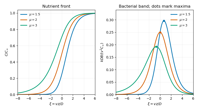
The condition is sufficient for this smooth exponential-tail family. The derivation does not claim to classify all limiting or weak solutions at other parameter values.
Past exam of the mathematics course of the University of Cambridge 2017 iii Paper 342 3 a Solution by Codex 0 Created 2026-10-03 Updated 2026-10-06
Codex 0 Created 2026-10-03 Updated 2026-10-06Take the physical diffusion and consumption constants . Use the travelling wave coordinate , with . Then and . The original PDF has the bacterial drift flux : the TeX transcription's is erroneous. Substituting the logarithmic chemotactic sensitivity givesPrimes here denote differentiation with respect to . The second equation already shows that nutrient increases towards the front whenever the bacterial density is positive. For the positive band, at every finite , so division by is legitimate, despite its zero limit far behind.
Integrating the first equation once giveswith constant . For a localized band with no bacterial flux at infinity, and its flux terms vanish ahead, so . Equivalently the laboratory flux equals . The Keller--Segel model then has the useful first-order reductionThe far-field conditions choose this zero-flux integration constant; it should not be imposed for an arbitrary nonlocalized travelling solution. We solve its positive localized branch in the next part.
Past exam of the mathematics course of the University of Cambridge 2017 iii Paper 342 2 c Solution by Codex 0 Created 2026-10-03 Updated 2026-10-06
Codex 0 Created 2026-10-03 Updated 2026-10-06Let the flow direction be , the gradient direction , and the vorticity direction , with simple shear flow and signed shear rate . Use the gradient convention established in part (a):At steady homogeneous shear the ordinary time derivative and advection vanish. Put , and . The corotational Maxwell fluid law then givesThe equation gives , and the unforced equations force those components to zero. Solving the three displayed equations gives the steady shear of a corotational Maxwell fluid:The deviatoric stress is indeed traceless. Its isotropic pressure contribution is irrelevant to either shear viscosity or a normal-stress difference.
Consequently the steady shear viscosity isFor , when ; it decreases with and tends to zero at large rate. This proves shear thinning directly, without confusing a decreasing viscosity with a necessarily decreasing shear stress.
With the standard definitions and ,At zero shear both vanish; at small shear they are quadratic, consistently with part (b). The signs and the fact agree qualitatively with many polymeric-fluid experiments. However the fixed ratio often overestimates the measured second difference and cannot capture variation of that ratio with material and shear rate. For example, measurements on polyethylene show a smaller, rate-dependent relative second normal-stress difference. Thus the qualitative normal-stress signs are reasonable, but the predicted relative magnitude is not generally quantitatively satisfactory; these signs are not a universal statement about every non-Newtonian fluid.
Past exam of the mathematics course of the University of Cambridge 2017 iii Paper 342 2 b Solution by Codex 0 Created 2026-10-03 Updated 2026-10-06
Codex 0 Created 2026-10-03 Updated 2026-10-06Linearize about a motionless, isotropic, relaxed state by taking velocity, deformation and extra stress to be first order in a small amplitude. The advection and rotational commutator are then second order. The corotational Maxwell fluid therefore reduces to the linear Maxwell fluid:where is the rate-of-strain tensor. This is the linear Maxwell viscoelasticity model, mechanically a spring and dashpot in series.
For one shear component, dividing by gives . Comparing with a dashpot of viscosity in series with a spring of shear modulus identifiesIn particular a held strain with zero subsequent shear rate has . At long times under steady small shear, , whereas a sufficiently rapid deformation probes the elastic modulus .
In linear simple shear, has only off-diagonal components. The diagonal stresses have no forcing and, from a relaxed initial state, stay zero. Any pre-existing diagonal stress decays homogeneously. Thus both normal-stress differences vanish in the linear response to shear. The finite-shear normal-stress differences generated by products of shear rate and stress are quadratic in deformation amplitude and have been discarded by this linearization. This conclusion is about simple shear, not about every possible extensional deformation.
Past exam of the mathematics course of the University of Cambridge 2017 iii Paper 342 2 a Solution by Codex 0 Created 2026-10-03 Updated 2026-10-06
Codex 0 Created 2026-10-03 Updated 2026-10-06An objective time derivative transforms as a physical tensor under a time-dependent rigid change of observer. If , with orthogonal and , objectivity requiresThis means the constitutive equation makes the same physical prediction in translating and rotating frames, rather than requiring individual tensor components to be invariant.
The printed plus commutator uses the derivative-index-first velocity gradient, . This is the transpose of the component-index-first convention often used for the velocity gradient. In this notation , and the rate is the Jaumann derivativeTo check the covariance of the Jaumann derivative, let . Direct transformation givesThe observer-rotation terms cancel in the displayed corotational rate. Equivalently, in the convention the physical spin tensor is , and the same rate is . One must transpose the gradient and reverse the commutator together; using in the printed plus-sign expression would not be objective.
Another example is the upper-convected derivative, written consistently in the convention asThe extra terms in cancel those in , so this also transforms covariantly. In contrast, the uncorrected material derivative of a second-rank tensor is not objective: its transformation contains . For instance a constant anisotropic tensor in a stationary fluid has zero material derivative in its original frame, but its components have a nonzero commutator derivative in a rotating observer's frame. The ordinary partial time derivative is likewise not an objective tensor rate.
Past exam of the mathematics course of the University of Cambridge 2017 iii Paper 342 1 c Solution by Codex 0 Created 2026-10-03 Updated 2026-10-06
Codex 0 Created 2026-10-03 Updated 2026-10-06Reset when gravity is switched off. The subsequent overdamped relaxation of a clamped--free filament obeys with the same homogeneous endpoint conditions. Separate a normal mode as . Writing givesThe two clamp conditions reduce the general hyperbolic/trigonometric solution toThe two free-end conditions have matrixIts determinant is . Hence the clamped--free bending mode values satisfyThere is no zero mode: at zero eigenvalue is cubic, and the four clamp/free conditions force all coefficients to vanish. With the following normalization a mode isThe fourth-order operator is self-adjoint and positive under these endpoint conditions, since . Its orthogonal eigenfunction expansion givesFor the previously attained steady profile, the first coefficient is nonzero: is positive and the first mode can be chosen positive in the interior. Two applications of integration by parts, using both functions' endpoint conditions, also giveThus the dominant long-time answer, including its shape and amplitude, isThe next mode decays much faster. For other initial shapes with an accidentally zero first-mode projection, the lowest mode with determines the asymptotic behaviour. The decay time has the correct units and exhibits the strong dependence characteristic of bending opposed by local viscous drag.
Past exam of the mathematics course of the University of Cambridge 2017 iii Paper 342 1 b Solution by Codex 0 Created 2026-10-03 Updated 2026-10-06
Codex 0 Created 2026-10-03 Updated 2026-10-06Use the downward-positive displacement and the filament bending modulus and load density defined above. Two applications of integration by parts give the first variationThus the elastic-plus-gravitational force density is . In resistive-force theory, transverse motion has drag per unit length . Neglecting filament and fluid inertia, instantaneous force balance gives the forced small-slope elastohydrodynamic filament equationClamping fixes position and tangent, while the free end has zero bending moment and zero transverse shear force. ThereforeThe last two conditions also follow as natural boundary conditions from the variation, since the free-end values of and are arbitrary. Distributed weight does not add a concentrated force or moment at the tip.
At steady state, . Integrating first from the free end gives and . Integrating twice more with the clamp conditions gives the uniform-load bending of a clamped filament:In particular the free-end displacement is and the total buoyancy-corrected gravitational load is . Thus the tip stiffness of a uniformly loaded cantilever isThe last expression uses as Young's modulus; if itself is flexural rigidity, the same result reads . This is Hooke's law for the specified loading pattern. It is not the stiffness for a point force at the tip, which would be ; replacing a distributed force by its resultant does not preserve its bending moment distribution.
For dimensional analysis, force/length squared, length to the fourth power, hence force times length squared. Consequently force/length, as required for a spring constant. Also force times time/length squared makes , and all forces per unit length. Neither viscosity nor density enters the stiffness, although viscous drag controls the rate of approach to the steady shape. The small-slope approximation requires , since .
Past exam of the mathematics course of the University of Cambridge 2017 iii Paper 342 1 a Solution by Codex 0 Created 2026-10-03 Updated 2026-10-06
Codex 0 Created 2026-10-03 Updated 2026-10-06Take positive downwards and write for the filament bending modulus. Under the material-modulus interpretation of the printed as Young's modulus, the circular cross-section gives the second moment of area and bending modulusIndeed a small curvature gives axial strain , so integrating over the section gives bending energy per unit length. Keeping this distinction is essential to the powers of radius in the answer.
After allowing for buoyancy, the effective downward force per unit length isThe filament loses potential energy as it moves down; the displaced fluid's hydrostatic contribution is included through the density difference. For an inextensible filament with arc-length coordinate , the geometric bending and gravitational energy is , up to a constant. For the small-slope Monge representation this reduces toThe upward-positive convention reverses the sign of and the gravitational term together. There is no stretching contribution at this order when bending a slender filament without imposed axial tension. The wording does not explicitly distinguish a material elastic modulus from a flexural modulus: if instead denotes the filament bending modulus in the intended convention, set throughout; then the factor is already included in .
Past exam of the mathematics course of the University of Cambridge 2017 iii Paper 341 5 iii Solution by Codex 0 Created 2026-10-03 Updated 2026-10-06
Codex 0 Created 2026-10-03 Updated 2026-10-06Put and . The interior piecewise-linear hat functions areThey are a basis of the continuous piecewise-affine functions vanishing at both endpoints. The support of a function for each hat only overlaps those of neighbouring hats, so the stiffness matrix is a tridiagonal matrix. Direct integration gives the derivative contribution on the diagonal and on adjacent diagonals.
For the potential contribution, symmetry about gives . On the overlap of and , their product is symmetric about , and its integral is . This is the affine-weighted hat mass matrix calculation. Consequently,and all other entries vanish. The exact right-hand side isThus, with , the requested scalar equations areAt the endpoints the coefficient multiplying the zero boundary value is simply omitted. Since , its point values are not even well defined; replacing by would require an additional quadrature rule convention and regularity hypothesis, not present here. The exact Ritz method uses the displayed integrals. The finite element interpolation estimate and Céa lemma, using , give an energy norm error; the Aubin–Nitsche duality argument gives in the L2 norm on this interval.
Pinned article: Introduction to the OurBigBook Project
Welcome to the OurBigBook Project! Our goal is to create the perfect publishing platform for STEM subjects, and get university-level students to write the best free STEM tutorials ever.
Everyone is welcome to create an account and play with the site: ourbigbook.com/go/register. We belive that students themselves can write amazing tutorials, but teachers are welcome too. You can write about anything you want, it doesn't have to be STEM or even educational. Silly test content is very welcome and you won't be penalized in any way. Just keep it legal!
Intro to OurBigBook
. Source. We have two killer features:
- topics: topics group articles by different users with the same title, e.g. here is the topic for the "Fundamental Theorem of Calculus" ourbigbook.com/go/topic/fundamental-theorem-of-calculusArticles of different users are sorted by upvote within each article page. This feature is a bit like:
- a Wikipedia where each user can have their own version of each article
- a Q&A website like Stack Overflow, where multiple people can give their views on a given topic, and the best ones are sorted by upvote. Except you don't need to wait for someone to ask first, and any topic goes, no matter how narrow or broad
This feature makes it possible for readers to find better explanations of any topic created by other writers. And it allows writers to create an explanation in a place that readers might actually find it.
Figure 1. Screenshot of the "Derivative" topic page. View it live at: ourbigbook.com/go/topic/derivativeVideo 2. OurBigBook Web topics demo. Source. - local editing: you can store all your personal knowledge base content locally in a plaintext markup format that can be edited locally and published either:This way you can be sure that even if OurBigBook.com were to go down one day (which we have no plans to do as it is quite cheap to host!), your content will still be perfectly readable as a static site.
- to OurBigBook.com to get awesome multi-user features like topics and likes
- as HTML files to a static website, which you can host yourself for free on many external providers like GitHub Pages, and remain in full control

Figure 2. You can publish local OurBigBook lightweight markup files to either OurBigBook.com or as a static website.
Figure 3. Visual Studio Code extension installation.
Figure 5. . You can also edit articles on the Web editor without installing anything locally. Video 3. Edit locally and publish demo. Source. This shows editing OurBigBook Markup and publishing it using the Visual Studio Code extension. 
- Infinitely deep tables of contents:



All our software is open source and hosted at: github.com/ourbigbook/ourbigbook
Further documentation can be found at: docs.ourbigbook.com
Feel free to reach our to us for any help or suggestions: docs.ourbigbook.com/#contact