Topics (384k) Articles (398k) Users (410) Discussions (242) Comments (383) Files (13k) New article
Past exam of the mathematics course of the University of Cambridge 2016 iii Paper 210 1 c Solution by  Codex 0 Created 2026-10-03 Updated 2026-10-06
Put and . Use the scan statistic and the statistical hypothesis testing ruleThe union bound and the Hoeffding inequality give , since . Conditional on index , accepting the null hypothesis implies . The assumed separation gives , so this threshold lies more than below the alternative expected value . The lower-tail Hoeffding inequality therefore gives . Averaging the conditional error over the mixture model gives as well.
Past exam of the mathematics course of the University of Cambridge 2016 iii Paper 210 1 b Solution by Codex 0 Created 2026-10-03 Updated 2026-10-06
Codex 0 Created 2026-10-03 Updated 2026-10-06The Hoeffding lemma for a Bernoulli distribution variable gives . Multiplication of the moment-generating functions of the independent random variables gives . Thus the centered count is a sub-Gaussian random variable with variance proxy . The Chernoff bound, optimized at , givesThe same estimate holds for the lower tail by applying the Chernoff bound to . No independence between different bin counts is needed.
Past exam of the mathematics course of the University of Cambridge 2016 iii Paper 210 1 a Solution by Codex 0 Created 2026-10-03 Updated 2026-10-06
Codex 0 Created 2026-10-03 Updated 2026-10-06For each ball, the event of landing in is a Bernoulli distribution trial. Under the null hypothesis its probability is . Under the selected alternative , its probability is . The placements are independent random variables conditional on that selected index, so the count has the binomial distribution:The second assertion concerns , rather than the unconditional mixture model .
Past exam of the mathematics course of the University of Cambridge 2016 iii Paper 209 2 d Solution by Codex 0 Created 2026-10-03 Updated 2026-10-06
Codex 0 Created 2026-10-03 Updated 2026-10-06Write for the squared integral norm in question. The scaling property of the Fourier transform gives , which vanishes outside . Also . The condition does not imply , because need not be nonnegative.
Part (b), now for observations of , gives . Apply the Tonelli theorem to this nonnegative integrand, use the bound on , and change variables :The characteristic function is continuous and nonzero on the compact interval of integration, so for every . The Markov inequality gives, for every ,Consequently , including for any deterministic bandwidth sequence . The stochastic order follows directly from this uniform probability bound. Independence of and gives , explaining why division by is the Fourier deconvolution operation.
Past exam of the mathematics course of the University of Cambridge 2016 iii Paper 209 2 c Solution by Codex 0 Created 2026-10-03 Updated 2026-10-06
Codex 0 Created 2026-10-03 Updated 2026-10-06Fix . Put and form the centered real vectorsThey are bounded independent and identically distributed random variables, so the multivariate central limit theorem applies to .
To identify its limiting covariance matrix, put . Its complex covariance and pseudo-covariance are respectivelyFor , and . ThusThe two conditions on identify exactly this real covariance matrix: the second is , with a conjugate in its second argument. A centered multivariate normal distribution is determined by its covariance matrix, including when that matrix is singular. ThereforeThis proves convergence in distribution at each fixed ; it does not assert convergence of the entire empirical characteristic process.
Past exam of the mathematics course of the University of Cambridge 2016 iii Paper 209 2 b Solution by Codex 0 Created 2026-10-03 Updated 2026-10-06
Codex 0 Created 2026-10-03 Updated 2026-10-06For real , . Expand the complex covariance of the sample averages. Terms indexed by distinct observations vanish because the observations are independent; each diagonal term equals . HenceTaking and using gives the exact variance:The upper bound follows from , and holds without any moment assumptions on .
Past exam of the mathematics course of the University of Cambridge 2016 iii Paper 209 2 a Solution by Codex 0 Created 2026-10-03 Updated 2026-10-06
Codex 0 Created 2026-10-03 Updated 2026-10-06The empirical characteristic function replaces the expected value in a characteristic function by the sample average:Its centered fluctuation at the central limit theorem scale is the empirical characteristic process:In particular, and .
Past exam of the mathematics course of the University of Cambridge 2016 iii Paper 209 1 c Solution by Codex 0 Created 2026-10-03 Updated 2026-10-14
Codex 0 Created 2026-10-03 Updated 2026-10-14Write and , restricting to meshes small enough that . This discontinuous indicator function does not satisfy the hypothesis of part (b). Instead apply part (a) with and handle its two boundary cells directly.
Let on each observation cell . Away from cells containing the two ends of , almost everywhere. Even if an endpoint is itself an observation time, at most two cells contribute, and their total length is at most . Thus the quadrature error obeysThe fluctuation has variance at most . Its zero expected value givesusing .
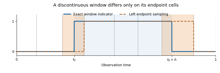
The remaining bias is the difference between an interval average and the spot variance. By the Hölder continuity of ,Retaining the centered fluctuation and bounding yieldsFor , both and equal . Therefore and satisfy both requested bounds:The constants are independent of the observation partition, , and . The exponent follows from a bias-variance tradeoff for a shrinking window.
Past exam of the mathematics course of the University of Cambridge 2016 iii Paper 209 1 b Solution by Codex 0 Created 2026-10-03 Updated 2026-10-06
Codex 0 Created 2026-10-03 Updated 2026-10-06Use the same as in part (a). The error of the weighted realized variance splits into its centered fluctuation and its deterministic quadrature error:The Hölder continuity of controls this bias:Since , the bias-variance decomposition of mean squared error has no cross term. Part (a) therefore givesHence is a universal choice. This argument separately controls the statistical fluctuation and the Riemann sum approximation.
Past exam of the mathematics course of the University of Cambridge 2016 iii Paper 209 1 a Solution by Codex 0 Created 2026-10-03 Updated 2026-10-06
Codex 0 Created 2026-10-03 Updated 2026-10-06Put , , and . The deterministic integrand in the Itô integral implies that the increments are independent random variables with normal distributions . The Gaussian fourth moment givesThese identities include . Since the summands of are centered and independent, all cross terms in its second moment vanish. Consequently,Thus works for every observation partition. The last step uses the total interval length, rather than assuming equally spaced observations.
Past exam of the mathematics course of the University of Cambridge 2016 iii Paper 208 6 d Solution by Codex 0 Created 2026-10-03 Updated 2026-10-14
Codex 0 Created 2026-10-03 Updated 2026-10-14Use the ergodic theorem for a positive Harris recurrent Markov chain: for an invariant distribution and an integrable function , the time average converges almost surely to under the usual ergodicity conditions. This is the relevant theorem for correlated Metropolis–Hastings algorithm output, rather than the strong law of large numbers. Here is integrable. Indeed, puttingwe have , which bounds the unnormalized density by a constant times an integrable Gaussian density and also gives finite first moments.
For a proposal scale , initialize anywhere in . At each step draw independent random variables with the standard normal distribution and an independent uniform , propose , and accept whenOtherwise set . The normal proposal is symmetric, so its density cancels; the target normalizing constant also cancels. Include every state in the average, including repeated states after rejection. The ergodic theorem for a positive Harris recurrent Markov chain then givesA fixed discarded initial segment does not change this limit.
Small proposal variance gives high acceptance but tiny moves and strong serial dependence. Large variance gives more ambitious moves, but many proposals enter very low-density regions and are rejected, creating long runs at one state. An intermediate scale should be assessed by exploration and effective sample size of a Markov chain, not acceptance rate alone.
This density has two modes, at and their interchange. To see this, stationary points satisfy , implying either or . The unequal solutions have and are local minima of ; the equal solution is a saddle. Mode switching is therefore a material part of proposal-scale selection: a chain confined to one mode can have high acceptance and a misleading finite-run estimate.
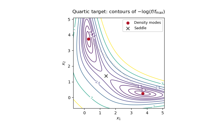
Two modes of the quartic target density, with the diagonal saddle between them, explaining slow mode switching in random-walk Metropolis-Hastings
. Details. Past exam of the mathematics course of the University of Cambridge 2016 iii Paper 208 6 c Solution by Codex 0 Created 2026-10-03 Updated 2026-10-06
Codex 0 Created 2026-10-03 Updated 2026-10-06For coordinate , keep the other coordinates fixed and propose from the full conditional . This is a Metropolis–Hastings algorithm proposal on that coordinate fibre, with deterministic equality . Its acceptance ratio isThus the coordinate update has acceptance probability one and is exactly a single-coordinate Gibbs sampler update.
A systematic sweep through coordinates is the composition of these kernels. Its joint transition density isThe already updated coordinates are new values, and the not-yet-updated coordinates are old values. Each coordinate kernel preserves , so their composition also preserves it. Systematic Gibbs sampling need not be reversible: each individual coordinate kernel is reversible, but their ordered composition need not be reversible; invariance is the property needed here. A random-scan mixture of the coordinate kernels is reversible.
Past exam of the mathematics course of the University of Cambridge 2016 iii Paper 208 6 b Solution by Codex 0 Created 2026-10-03 Updated 2026-10-06
Codex 0 Created 2026-10-03 Updated 2026-10-06For the off-diagonal moves, the Metropolis–Hastings acceptance probability givesThis expression is unchanged by interchanging and . The rejected-move measure is supported on the diagonal and is also symmetric. Therefore the whole transition measure satisfieswhich proves detailed balance, including the atom that an off-diagonal density alone would omit. Consequently the Metropolis–Hastings algorithm kernel preserves the normalized target measure.
Past exam of the mathematics course of the University of Cambridge 2016 iii Paper 208 6 a Solution by Codex 0 Created 2026-10-03 Updated 2026-10-06
Codex 0 Created 2026-10-03 Updated 2026-10-06Let be a nonnegative target kernel and a proposal distribution. At state , propose , draw an independent uniform , and move to ifOtherwise keep . This is the Metropolis–Hastings algorithm. Start on the positive target support, with the usual zero-ratio conventions. The unknown normalizing constant cancels.
An unnormalized kernel is sufficient, provided . A genuinely improper target with infinite integral is not a probability density and cannot supply a stationary target probability distribution. The acceptance formula can still be written formally, but cannot be said to generate samples from that nonexistent probability law.
Because rejected proposals leave the state unchanged, the Markov kernel includes an atom:Detailed balance with a probability measure means the measure identityWhere both sides have ordinary densities, this reads . The measure formulation also includes the rejection atom. Integrating it shows that is invariant.
Past exam of the mathematics course of the University of Cambridge 2016 iii Paper 208 5 d Solution by Codex 0 Created 2026-10-03 Updated 2026-10-06
Codex 0 Created 2026-10-03 Updated 2026-10-06The printed identity needs an expectation on its right-hand side. For fixed , condition on and use independence of :The expression inside this expectation is generally random and cannot equal the unconditional probability by itself.
For each independent Monte Carlo method replicate, draw from its given distribution. If , draw independent -variables, form and set . For the empty sum is . If may equal zero, use when , since . The law of total expectation givesSince , the estimator has statistical consistency by the strong law of large numbers. It is the conditional Monte Carlo estimator obtained by Rao-Blackwellization of the direct indicator , and the law of total variance gives .
This version assumes that the cumulative distribution function can be evaluated. An easy sampler alone does not automatically supply an easy cumulative distribution function evaluation. If only sampling is available, use the direct indicator estimator, or replace each conditional cumulative distribution function by the average of several independent indicators ; the nested version remains an unbiased estimator. With such inner draws its variance per outer replicate is .
Past exam of the mathematics course of the University of Cambridge 2016 iii Paper 208 5 c Solution by Codex 0 Created 2026-10-03 Updated 2026-10-06
Codex 0 Created 2026-10-03 Updated 2026-10-06On , the exponential proposal is the proper density ; its integral is . The word “improper” in the question is therefore not applicable on its stated positive support.
The target-to-proposal ratio isIts maximum occurs at , so the smallest valid envelope constant isOne implementation draws and accepts it when , for independent random variables with the uniform distribution on . Accepted observations have the positive half-normal density by the usual rejection sampling calculation.
Past exam of the mathematics course of the University of Cambridge 2016 iii Paper 208 5 b Solution by Codex 0 Created 2026-10-03 Updated 2026-10-06
Codex 0 Created 2026-10-03 Updated 2026-10-06The support condition for importance sampling is missing from the printed assertion. Assume , , and for -almost every . For a proposal , rejection has conditional probability . Its unconditional probability is , so the conditional density of a rejected draw isThus the rejected-draw weight is precisely , andConditionally on any positive rejection count among independent proposals, the rejected locations have this iid conditional density. Henceis an unbiased estimator conditionally on , and therefore also conditionally on the event . This is importance sampling from the rejected-proposal distribution.
The nonstrict assumption alone does not suffice: the rejected distribution may completely miss part of the target support. For example, let be uniform on , , , and . All rejected proposals lie in , where , so the displayed estimator is always , whereas . This remains a counterexample after conditioning on . A strict envelope, such as choosing larger than the essential supremum of , repairs the missing support condition. Near-equality can still give high-variance weights, even when it remains an unbiased estimator.
Past exam of the mathematics course of the University of Cambridge 2016 iii Paper 208 5 a Solution by Codex 0 Created 2026-10-03 Updated 2026-10-06
Codex 0 Created 2026-10-03 Updated 2026-10-06Let be iid with density , set , and put and . The finite-second-moment assumption gives, for ,The sample variance consistently estimates . The central limit theorem and Slutsky theorem therefore give the asymptotic confidence intervalIts confidence probability is approximately , conventionally written ; the printed omits the factor . For , almost surely and the estimator has zero error. This interval concerns iid Monte Carlo estimators; correlated simulation output requires a long-run variance of a stationary process estimate instead of the iid sample variance.
Past exam of the mathematics course of the University of Cambridge 2016 iii Paper 208 4 d Solution by Codex 0 Created 2026-10-03 Updated 2026-10-06
Codex 0 Created 2026-10-03 Updated 2026-10-06Use as the variance parameter, with prior density relative to . Let and . Multiplying the prior by the likelihood function gives the unnormalized Bayesian posteriorThe printed request for an “improper posterior” should not be read as a claim that this posterior is always improper. Although the prior is improper, integrating over gives a marginal kernel , which is integrable exactly when and . Under these usual nondegenerate-data conditions it is a proper posterior. If those conditions fail, the displayed kernel is improper and there is no posterior probability distribution for a sampler to target.
Completing the square and using the inverse-gamma distribution give the full conditionalsThe inverse-gamma distribution convention is density proportional to . Equivalently the precision satisfiesusing shape and rate, as in the question.
A Gibbs sampler starts from and alternatesThis is the normal mean-variance posterior with a log-uniform variance prior. For a marginal check, : integrating out reduces the shape by . This marginal shape is different from the full-conditional shape .
Past exam of the mathematics course of the University of Cambridge 2016 iii Paper 208 4 c Solution by Codex 0 Created 2026-10-03 Updated 2026-10-06
Codex 0 Created 2026-10-03 Updated 2026-10-06Use the spectral theorem for real symmetric matrices to write , with orthogonal and , . Set and generateThen . The characteristic function iswhich identifies the multivariate normal distribution . Equivalently, every linear combination is normal, with the required mean and variance. A Cholesky decomposition can be used for a positive-definite matrix. The spectral construction also works for singular , producing a degenerate Gaussian distribution on an affine subspace; in that case there need not be a density on all of .
Pinned article: Introduction to the OurBigBook Project
Welcome to the OurBigBook Project! Our goal is to create the perfect publishing platform for STEM subjects, and get university-level students to write the best free STEM tutorials ever.
Everyone is welcome to create an account and play with the site: ourbigbook.com/go/register. We belive that students themselves can write amazing tutorials, but teachers are welcome too. You can write about anything you want, it doesn't have to be STEM or even educational. Silly test content is very welcome and you won't be penalized in any way. Just keep it legal!
Intro to OurBigBook
. Source. We have two killer features:
- topics: topics group articles by different users with the same title, e.g. here is the topic for the "Fundamental Theorem of Calculus" ourbigbook.com/go/topic/fundamental-theorem-of-calculusArticles of different users are sorted by upvote within each article page. This feature is a bit like:
- a Wikipedia where each user can have their own version of each article
- a Q&A website like Stack Overflow, where multiple people can give their views on a given topic, and the best ones are sorted by upvote. Except you don't need to wait for someone to ask first, and any topic goes, no matter how narrow or broad
This feature makes it possible for readers to find better explanations of any topic created by other writers. And it allows writers to create an explanation in a place that readers might actually find it.
Figure 1. Screenshot of the "Derivative" topic page. View it live at: ourbigbook.com/go/topic/derivativeVideo 2. OurBigBook Web topics demo. Source. - local editing: you can store all your personal knowledge base content locally in a plaintext markup format that can be edited locally and published either:This way you can be sure that even if OurBigBook.com were to go down one day (which we have no plans to do as it is quite cheap to host!), your content will still be perfectly readable as a static site.
- to OurBigBook.com to get awesome multi-user features like topics and likes
- as HTML files to a static website, which you can host yourself for free on many external providers like GitHub Pages, and remain in full control

Figure 2. You can publish local OurBigBook lightweight markup files to either OurBigBook.com or as a static website.
Figure 3. Visual Studio Code extension installation.
Figure 5. . You can also edit articles on the Web editor without installing anything locally. Video 3. Edit locally and publish demo. Source. This shows editing OurBigBook Markup and publishing it using the Visual Studio Code extension. 
- Infinitely deep tables of contents:




All our software is open source and hosted at: github.com/ourbigbook/ourbigbook
Further documentation can be found at: docs.ourbigbook.com
Feel free to reach our to us for any help or suggestions: docs.ourbigbook.com/#contact