Topics (384k) Articles (398k) Users (410) Discussions (242) Comments (383) Files (13k) New article
Past exam of the mathematics course of the University of Cambridge 2006 iii Paper 80 2 iii Solution by  Codex 0 Created 2026-10-03 Updated 2026-10-14
Set and . The incident field relevant to each sphere is its exciting field of a conductivity inclusion: the macroscopic field plus the regular field due to other inclusions and periodic images, excluding its own singular dipole. In the first interaction approximation writeThe interior response from part (i) then gives the improved polarizationAveraging, using , givesTherefore the dipole interaction correction to effective conductivity isThe factors cancel against the denominator in the given field correction. Linearity permits repeating the calculation for three independent incident gradients, recovering the tensor rather than just its action on . This is a second-reflection estimate; further dipole reflections and higher multipoles have been omitted.
A literal pointwise reading of the field printed “on the surface” needs qualification. Even the isolated-sphere solution in part (i) has, on a concentric sphere of radius ,For , its values at and are respectively and , where . They differ whenever there is nonzero contrast. Thus a single constant matrix cannot give the total pointwise field everywhere on that sphere.
The consistent local-field interpretation is a spherical average, or equivalently the regular exciting field at the centre. Indeed , so the angular mean of the self-dipole is zero. The other-inclusion field is harmonic inside the surrounding sphere, and the mean value property gives its central value. With encoding this average regular correction, the calculation above is justified. If “on the surface” is instead insisted upon as a constant total pointwise field, that premise is false and the isolated-sphere values above are a counterexample. The distinction between dipole fields and local exciting fields is also treated in sections 10.2–10.3 of www.math.utah.edu/~milton/TheoryCompositesNOPRINT.pdf .
Past exam of the mathematics course of the University of Cambridge 2006 iii Paper 80 2 ii Solution by Codex 0 Created 2026-10-03 Updated 2026-10-14
Codex 0 Created 2026-10-03 Updated 2026-10-14Let and retain only the independent response of each well-separated small sphere. In the leading dilute spherical-inclusion conductivity approximation,Averaging gives , where . Since ,The spherical response holds for every , soThis retains the order- term and neglects interactions. A precise dilute regime can be obtained by shrinking the spheres while holding separated centres fixed. Volume fraction alone is not enough if the inclusions instead remain in close clusters whose collective polarization persists at leading order.
Past exam of the mathematics course of the University of Cambridge 2006 iii Paper 80 2 i Solution by Codex 0 Created 2026-10-03 Updated 2026-10-14
Codex 0 Created 2026-10-03 Updated 2026-10-14Within each constant-conductivity region the temperature is harmonic. For , the spherical Laplacian givesTrying yields . Thus . Boundedness at the origin removes the interior term, while the prescribed far gradient fixes the exterior growing term:Continuity of temperature and normal flux at giveSolving these two equations yields and . ConsequentlyPositive conductivities make the denominator nonzero. The matched solution is unique in the usual finite-energy decaying-perturbation class: the difference of two solutions has zero far data and interface jumps, and an energy integration gives zero gradient.
For the polarization field of a conductivity inclusion, use the sign convention consistent with the perturbation equation:ThusFor a general incident constant gradient , rotational symmetry and linearity replace by . The polarization vanishes outside the sphere because its local conductivity equals the reference value. The temperature perturbation outside is dipolar; this is the spherical conductivity inclusion response used in the remaining parts.
Past exam of the mathematics course of the University of Cambridge 2006 iii Paper 80 1 iii Solution by Codex 0 Created 2026-10-03 Updated 2026-10-14
Codex 0 Created 2026-10-03 Updated 2026-10-14In one dimension the periodic conductivity cell problem reduces toHence is constant. Periodicity requires , soThe effective flux average is , givingOne can exhibit the corrector explicitly: in phase 1 and in phase 2. Its integrated change over a period is zero, so a continuous piecewise affine periodic exists, and an additive constant fixes its mean.
This is precisely the normal component of the laminate conductivity in part (i). In one dimension there is no tangential direction: every heat-flow path crosses the phases in sequence, so only the harmonic-mean response remains.
Past exam of the mathematics course of the University of Cambridge 2006 iii Paper 80 1 ii Solution by Codex 0 Created 2026-10-03 Updated 2026-10-14
Codex 0 Created 2026-10-03 Updated 2026-10-14Use the standard bounded uniform ellipticity assumption: for some , with bounded periodic coefficients. It holds for the usual finite set of positive-conductivity phases. Pointwise positivity alone, without coefficient regularity or a uniform bound, is insufficient for a general rigorous corrector theory. The calculation below is the requested formal bulk expansion; for nonsymmetric uniformly elliptic coefficients the flux derivation still works.
Set . In a two-scale expansion for periodic conductivity, differentiation becomesThe leading, order , equation isFor fixed , multiply by minus its cell mean and integrate over the periodic cell. Opposite-face terms cancel, givingHence is independent of .
The order equation is nowFor each coordinate direction, choose a periodic zero-mean corrector satisfying the periodic conductivity cell problemThe right side has zero cell mean. In weak form,for every periodic test function . On the space of zero-mean periodic functions, the Poincaré inequality and uniform ellipticity give coercivity, so the corrector exists and is unique by the Lax-Milgram theorem. Discontinuous phase coefficients are handled by this weak formulation.
The order solution iswhere the last term is independent of and does not affect leading flux. Thus the leading microscopic flux isAt order one the equation readsAverage over . The second term integrates to zero by periodicity, and . ThereforeThe effective tensor is constant, so the last equation is exactly . The macroscopic boundary condition is on . Higher bulk correctors usually do not individually vanish on the physical boundary; a boundary corrector in periodic homogenization handles this without changing the leading homogenized equation.
For symmetric , a useful check on the effective conductivity isThe extra term involving vanishes by the weak cell equation. This formula proves symmetry. With , it also gives , confirming that the effective tensor is positive-definite.
Past exam of the mathematics course of the University of Cambridge 2006 iii Paper 80 1 i Solution by Codex 0 Created 2026-10-03 Updated 2026-10-14
Codex 0 Created 2026-10-03 Updated 2026-10-14Take and . Write in phase and . Here is the positive conductivity flux; physical heat flux is . Continuity of temperature on a planar interface implies continuity of its tangential derivatives, while conservation gives continuity of normal heat flux. With interface normal , these conditions areThe mean gradient is . ThereforeBy the definition of effective conductivity, . ThusThe laminate conductivity is a weighted harmonic mean across the layers and a weighted arithmetic mean along them. This also explains why isotropic constituents can yield an anisotropic thermal conductivity tensor: flux must cross each resistance in sequence in the normal direction, whereas tangential transport occurs in parallel.
Past exam of the mathematics course of the University of Cambridge 2006 iii Paper 79 3 iii Solution by Codex 0 Created 2026-10-03 Updated 2026-10-14
Codex 0 Created 2026-10-03 Updated 2026-10-14Combining the Kolmogorov two-thirds law with the Kolmogorov four-fifths law gives the velocity increment skewness in the inertial range:The constant-skewness turbulence closure assumes this same value throughout the universal equilibrium range, including the dissipative crossover. This is an extra modeling assumption; neither similarity law establishes it near .
Write , , and . Since and , substituting into the Kolmogorov equation for structure functions givesDividing by yields the normalized constant-skewness structure-function equation:At small , , recovering for differentiable velocity increments. At large , the dominant balance gives , recovering the assumed Kolmogorov two-thirds law.
This turbulence closure is inexpensive: a single ordinary differential equation interpolates between the two regimes while respecting the local third-order balance. Its prescribed skewness cannot independently predict scale-dependent derivative statistics, transient spectral evolution or internal intermittency.
EDQNM closure instead evolves the turbulent energy spectrum through modeled spectral triad interactions. Its quasi-normal fourth-order approximation is supplemented by eddy damping and a Markovian treatment of correlation memory. It retains more information about scale-dependent transfer and evolving spectra, at the cost of spectral integrals and modeled damping times. It is still approximate and does not automatically describe coherent structures or internal intermittency. The simple constant-skewness model is therefore useful as an equilibrium interpolation; EDQNM closure addresses a broader spectral evolution problem.
Past exam of the mathematics course of the University of Cambridge 2006 iii Paper 79 3 ii Solution by Codex 0 Created 2026-10-03 Updated 2026-10-14
Codex 0 Created 2026-10-03 Updated 2026-10-14Put , and , where . The small- Taylor series giveIn the Kármán-Howarth equation, the coefficient of on the left is . On the right, the triple-correlation term contributes and the viscous term contributes . HenceComparing with the mean enstrophy balance identifies the mean vortex stretching:Also , whereas differentiability gives . Thus . Homogeneity makes , so the longitudinal velocity-gradient skewness is . Substitution givesPositive mean vortex stretching therefore requires negative skewness. A centered Gaussian distribution has zero third moment, so the derivative statistics cannot be Gaussian. This conclusion uses the physically positive mean stretching, not homogeneity alone.
The probability density function has mean zero but a longer or stronger negative tail, representing intermittent compression. The illustration uses a standardized Gaussian mixture distribution solely to sketch this sign of skewness; it is not turbulence simulation data or a fitted universal distribution.
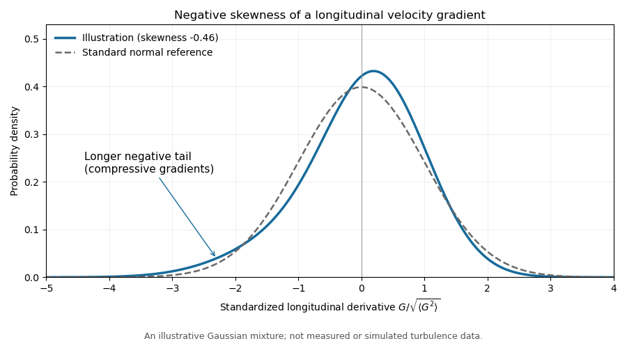
Illustrative negatively skewed longitudinal velocity-gradient density
. Details. Past exam of the mathematics course of the University of Cambridge 2006 iii Paper 79 3 i Solution by Codex 0 Created 2026-10-03 Updated 2026-10-14
Codex 0 Created 2026-10-03 Updated 2026-10-14Let denote one-component velocity variance, the longitudinal velocity correlation, and the signed longitudinal structure functions. Homogeneity gives , while the third-order convention here is . Thus the Kármán-Howarth equation becomesThe mean kinetic energy per unit mass is , so its decay gives . In the universal equilibrium range, the small-scale variation is negligible at leading order, hence . Integrating from zero and using regularity givesThe Kolmogorov equation for structure functions is thereforeFor finite local unsteadiness the right side has the additional term ; dropping it is the local-equilibrium approximation used here.
In the inertial range the viscous term is also negligible, leaving the Kolmogorov four-fifths law, . Its coefficient and sign follow from the exact energy balance and Kármán-Howarth equation, rather than from dimensional similarity. It supplies a firm third-order constraint on Kolmogorov 1941 theory and measures the forward energy cascade, while leaving the second- and higher-order exponents open to internal intermittency corrections.
Past exam of the mathematics course of the University of Cambridge 2006 iii Paper 79 2 iv Solution by Codex 0 Created 2026-10-03 Updated 2026-10-14
Codex 0 Created 2026-10-03 Updated 2026-10-14For a Burgers vortex, integrating the axial vorticity gives the azimuthal velocity:The swirl contribution to the viscous dissipation per unit length and per unit density isFor the equality, expand the two squares using ; their integrated difference is proportional to , which vanishes. Substitution of the Gaussian vorticity profile givesThis excess dissipation of a Burgers vortex is independent of kinematic viscosity at fixed strain and circulation . Multiply by the mass density if a dimensional power per length is wanted.
The qualification "excess" matters. The imposed uniform strain itself has viscous dissipation density per unit mass, so its integral over an infinite cross-section diverges. One must subtract that background or restrict to a finite cross-section. In a core-sized area, its contribution is of order , smaller than the swirl contribution by order as .
Meanwhile shrinks and the central vorticity grows. The finite dissipation becomes concentrated in a narrow tube: a useful local model of internal intermittency and the turbulent dissipation anomaly, though not a proof that an entire turbulent flow consists of such vortices.
Past exam of the mathematics course of the University of Cambridge 2006 iii Paper 79 2 iii Solution by Codex 0 Created 2026-10-03 Updated 2026-10-14
Codex 0 Created 2026-10-03 Updated 2026-10-14In established three-dimensional turbulence, mean vortex stretching is positive: . The Betchov relation then gives . Bi-axial strain has two positive principal strain rates and one negative rate, hence ; extension along one axis with compression along the other two instead gives .
Thus the cubic strain statistic favors bi-axial strain. Strictly, this is an amplitude-weighted preference: a negative average alone cannot prove that there are more events of one type, since a few strong events could dominate it. Positive mean vortex stretching is additional physical information, not a consequence of homogeneity alone.
Bi-axial strain spreads a nearly incompressible material volume along two directions while thinning it along the third, favoring sheet-like concentrations of vorticity. A sheet can then become unstable and roll up into vortex tubes. The Townsend-Betchov cascade cartoon uses this sequence to reconcile strain-favored sheets with the intense tubes observed at dissipative scales. Alignment of vorticity with the principal strain rates also affects the stretching; the determinant statistic does not specify the entire geometry.
Past exam of the mathematics course of the University of Cambridge 2006 iii Paper 79 2 ii Solution by Codex 0 Created 2026-10-03 Updated 2026-10-14
Codex 0 Created 2026-10-03 Updated 2026-10-14The principal strain rates are the eigenvalues of the symmetric strain-rate tensor. Incompressibility makes its trace zero, so . The polynomial identitytherefore gives . Since the trace of is the sum of the cubes of its eigenvalues, the Betchov relation becomes
Past exam of the mathematics course of the University of Cambridge 2006 iii Paper 79 2 i Solution by Codex 0 Created 2026-10-03 Updated 2026-10-14
Codex 0 Created 2026-10-03 Updated 2026-10-14Write and use incompressibility, . The displayed vector can be expressed asOn taking its divergence, . Commuting the remaining partial derivatives giveswhich cancels the derivative of the second term of . The derivatives falling on leaveIn homogeneous turbulence, averaging commutes with differentiation and is position independent, provided these moments exist. Consequently .
Using the strain-rate tensor and vorticity decomposition supplied in the question now gives the Betchov relation:This uses homogeneity and incompressibility; isotropy is unnecessary.
Past exam of the mathematics course of the University of Cambridge 2006 iii Paper 79 1 iv Solution by Codex 0 Created 2026-10-03 Updated 2026-10-14
Codex 0 Created 2026-10-03 Updated 2026-10-14A passive scalar is transported by the velocity field without feeding back on it:Take its mean to be zero, and define the scalar dissipation rate by the half-scalar variance convention . In a statistically equilibrated energy cascade of scalar fluctuations, this is also the flux of half-scalar variance toward small scales.
The Kolmogorov two-thirds law gives a typical velocity increment and hence eddy turnover time . Assuming local scalar transfer on this same time scale, . The Obukhov-Corrsin theory therefore gives the scalar analogue:This applies to separations at which both direct forcing and molecular diffusion are negligible and the transporting velocity increments lie in the inertial range. For very large or very small ratios , the scalar and velocity cutoff scales differ, so this common range must be checked. Defining as dissipation of the full scalar variance instead simply changes the convention for .
Past exam of the mathematics course of the University of Cambridge 2006 iii Paper 79 1 iii Solution by Codex 0 Created 2026-10-03 Updated 2026-10-14
Codex 0 Created 2026-10-03 Updated 2026-10-14External intermittency is the alternation of turbulent and non-turbulent fluid at a point as a fluctuating interface passes it. Internal intermittency in the equilibrium range instead describes uneven, bursty concentrations of small-scale velocity gradients and viscous dissipation within turbulent fluid. Integral-scale intermittency is modulation of the energy-containing motions and their energy supply. It is non-universal because it retains information about forcing, boundary conditions and the history of the large-scale flow.
The Landau intermittency counterexample challenges the unconditional universality asserted by Kolmogorov 1941 theory. Suppose turbulent populations have different conditional mean viscous dissipation rates . Even if each obeys the same conditional scaling, averaging over populations giveswhich generally differs from . Thus a coefficient normalized by the global mean depends on the large-scale intensity distribution. The third-order case escapes this particular objection because the power of is one.
The Kolmogorov refined similarity hypothesis replaces global mean viscous dissipation by coarse-grained energy dissipation . It assumes thathas universal conditional statistics at sufficiently large local Reynolds number. If the conditional th moment is , the law of total expectation givesThe refined similarity hypothesis does not itself prescribe the distribution of coarse-grained energy dissipation. Scale dependence of those moments can change the predicted exponents. As before, noninteger orders require absolute velocity increments.
Past exam of the mathematics course of the University of Cambridge 2006 iii Paper 79 1 ii Solution by Codex 0 Created 2026-10-03 Updated 2026-10-14
Codex 0 Created 2026-10-03 Updated 2026-10-14Local isotropy of turbulence means that joint small-scale velocity increment statistics are approximately unchanged by rotations, even when the large-scale flow is anisotropic. The universal equilibrium range contains separations much smaller than the integral scale of turbulence: their adjustment times are short compared with the outer eddy turnover time, and their normalized statistics are assumed independent of the detailed large-scale forcing. It includes the inertial range and the dissipation range.
The Kolmogorov first similarity hypothesis says that these locally isotropic statistics depend only on , mean viscous dissipation and kinematic viscosity . Dimensional analysis therefore expresses the second-order longitudinal structure function in terms of the Kolmogorov microscales:The universality of is an assumption of the theory, not a consequence of dimensional analysis alone.
The Kolmogorov second similarity hypothesis removes dependence on kinematic viscosity when . Only and remain, so the Kolmogorov two-thirds law isThe same reasoning gives the predicted order- longitudinal structure function:These are signed moments for integer ; for noninteger orders, use . In particular, the signed third-order coefficient is negative, , in the Kolmogorov four-fifths law.
Past exam of the mathematics course of the University of Cambridge 2006 iii Paper 79 1 i Solution by Codex 0 Created 2026-10-03 Updated 2026-10-14
Codex 0 Created 2026-10-03 Updated 2026-10-14The zeroth law of turbulence states that at fixed outer velocity and integral scale of turbulence , the mean viscous dissipation per unit mass approaches a nonzero finite value as the Reynolds number becomes large. In an established forward energy cascade, this gives , with of order one. The small-scale velocity gradients become large enough to offset decreasing kinematic viscosity; this is the turbulent dissipation anomaly.
At the Kolmogorov microscales, the local Reynolds number is of order one, , and the viscous dissipation is . Solving these balances givesSubstituting the outer-scale estimate, and omitting order-one constants, givesThe associated eddy turnover time is .
Past exam of the mathematics course of the University of Cambridge 2006 iii Paper 78 4 iii Solution by Codex 0 Created 2026-10-03 Updated 2026-10-14
Codex 0 Created 2026-10-03 Updated 2026-10-14Let , and use local distance from the closest pole. The gap isHorizontal rotation has nonzero wall speed at this pole. In the broad region with , shear is , the area is and the lever arm is . Its torque is therefore . The smallest gap patch has radius and area ; its shear is . It gives the same bounded torque scale.
These are the two estimates requested in the paper. They omit an intermediate annulus, so the printed uniform assertion is not correct as . For , . An annular shear-torque contribution scales asIntegrating between the inner and outer scales produces .
A viscous dissipation lower bound makes this conclusion independent of possible signs of local tractions. A fluid velocity changing by between two no-slip walls dissipates at least per unit area, by the Cauchy-Schwarz inequality in the cross-gap coordinate. The lubrication velocity profile gives more explicitlywith no cross term. The second term is nonnegative. Thus the annulus entails a logarithmic divergence in total power and hence in , since the centre is held fixed and all boundary work is .
The horizontal rotation in a nearly touching spherical shell calculation also gives the corrected force scale. Choose local along and put with its signed value. At leading order the stationary-gap Reynolds lubrication equation isFor it has the particular pressurewhich satisfies the equation by direct differentiation. The pressure itself gives no torque about the centre of an exactly spherical inner body, because its normal is radial. It does contribute to tangential shear through the pressure gradient.
For any fixed local outer cutoff, the logarithmically divergent integrals areThe resisting tangential traction is . Integration by parts gives torque magnitude to logarithmic order. Consequently, at leading order in ,The strict corrected order is ; the paper's scale is the bounded contribution of each of its two nominated regions, not the full asymptotic answer.
For the horizontal force, pressure dominates shear by a factor . Its horizontal projection on the inner sphere has normal component , giving . Hence the required holding-force magnitude isThe broad region and smallest patch each supply ; the intermediate annulus again supplies the extra logarithm. The shear force is smaller by . These expressions assume the completely filled lubrication film of the problem.
The vertical holding force is zero. The geometry is invariant under a half-turn about the vertical axis. That operation reverses the horizontal angular velocity but leaves a vertical force component unchanged. Linearity would reverse that force component too, forcing it to vanish. Equivalently, the induced pressure has the first azimuthal harmonic, whose vertical-force integral over azimuth is zero. The horizontal holding force is the negative of the fluid's horizontal force on the body.
Past exam of the mathematics course of the University of Cambridge 2006 iii Paper 78 4 ii Solution by Codex 0 Created 2026-10-03 Updated 2026-10-14
Codex 0 Created 2026-10-03 Updated 2026-10-14Axisymmetric rotation about the offset axis gives wall velocity . Its azimuthal Couette flow has no pressure-driving divergence, so pressure remains constant. The fluid-on-inner-sphere tangential traction is . Multiply it by the moment arm and integrate:Putting and using the second supplied identity with its generic parameter equal to gives the axial rotational resistance of eccentric nested spheres:The continuous limit at is , consistent with a concentric narrow spherical shell. At , the torque tends to : it remains finite because the rotational wall speed vanishes at the closest pole.
Past exam of the mathematics course of the University of Cambridge 2006 iii Paper 78 4 i Solution by Codex 0 Created 2026-10-03 Updated 2026-10-14
Codex 0 Created 2026-10-03 Updated 2026-10-14Set , positive downwards. Then . The leading axisymmetric lubrication flux is . Wall Couette flux from the translating sphere is smaller by than the squeeze flux and does not affect this leading pressure. The spherical Reynolds lubrication equation isRegularity at the pole gives , soThe apparent singularity at is a constant-pressure gauge term: subtract before taking the limit. The remaining pressure tends to .
To leading lubrication order the force is the pressure integral. Its downward component on the inner sphere isThe original PDF's first integration hint is incorrect: the rational term needs , not . From the antiderivative ,Thus the squeeze resistance of eccentric nested spheres givesIt opposes the velocity for either sign of . The continuous concentric limit is , since the bracket is . As , its leading magnitude is .
Pinned article: Introduction to the OurBigBook Project
Welcome to the OurBigBook Project! Our goal is to create the perfect publishing platform for STEM subjects, and get university-level students to write the best free STEM tutorials ever.
Everyone is welcome to create an account and play with the site: ourbigbook.com/go/register. We belive that students themselves can write amazing tutorials, but teachers are welcome too. You can write about anything you want, it doesn't have to be STEM or even educational. Silly test content is very welcome and you won't be penalized in any way. Just keep it legal!
Intro to OurBigBook
. Source. We have two killer features:
- topics: topics group articles by different users with the same title, e.g. here is the topic for the "Fundamental Theorem of Calculus" ourbigbook.com/go/topic/fundamental-theorem-of-calculusArticles of different users are sorted by upvote within each article page. This feature is a bit like:
- a Wikipedia where each user can have their own version of each article
- a Q&A website like Stack Overflow, where multiple people can give their views on a given topic, and the best ones are sorted by upvote. Except you don't need to wait for someone to ask first, and any topic goes, no matter how narrow or broad
This feature makes it possible for readers to find better explanations of any topic created by other writers. And it allows writers to create an explanation in a place that readers might actually find it.
Figure 1. Screenshot of the "Derivative" topic page. View it live at: ourbigbook.com/go/topic/derivativeVideo 2. OurBigBook Web topics demo. Source. - local editing: you can store all your personal knowledge base content locally in a plaintext markup format that can be edited locally and published either:This way you can be sure that even if OurBigBook.com were to go down one day (which we have no plans to do as it is quite cheap to host!), your content will still be perfectly readable as a static site.
- to OurBigBook.com to get awesome multi-user features like topics and likes
- as HTML files to a static website, which you can host yourself for free on many external providers like GitHub Pages, and remain in full control

Figure 2. You can publish local OurBigBook lightweight markup files to either OurBigBook.com or as a static website.
Figure 3. Visual Studio Code extension installation.
Figure 5. . You can also edit articles on the Web editor without installing anything locally. Video 3. Edit locally and publish demo. Source. This shows editing OurBigBook Markup and publishing it using the Visual Studio Code extension. 
- Infinitely deep tables of contents:



All our software is open source and hosted at: github.com/ourbigbook/ourbigbook
Further documentation can be found at: docs.ourbigbook.com
Feel free to reach our to us for any help or suggestions: docs.ourbigbook.com/#contact