
Negative binomial exponential family Created 2026-09-24 Updated 2026-09-24
For fixed positive integer , the failures-before-the-th-success distribution is a one-parameter exponential family withand carrier .
Exponential-family deviance Created 2026-09-24 Updated 2026-10-14
Inverse Gaussian distribution Created 2026-09-24 Updated 2026-09-24
For an expected value parameter and a shape parameter , the inverse Gaussian distribution has probability density functionIts mean is and its variance is .
Cumulant function of an exponential family Created 2026-09-24 Updated 2026-10-07
Natural parameter of an exponential family Created 2026-09-24 Updated 2026-10-07
Finite subgroup of a field multiplicative group is cyclic Created 2026-09-24 Updated 2026-11-05
Tail integral formula for moments Created 2026-09-24 Updated 2026-11-05
For and a real random variable , the tail integral formula for moments isvalid even if both sides are infinite. Pointwise, ; Tonelli theorem interchanges this nonnegative integral with expectation. Replacing by does not change the integral, since their difference is confined to the at most countably many atoms of the distribution. For an exponential random variable of rate , the formula at gives .
Variance of a sample mean Created 2026-09-24 Updated 2026-10-14
Let be an IID sample of real-valued random variables with finite expected value and finite variance , where . Its sample mean satisfiesLinearity of expectation gives the first identity. The variance of a sum and vanishing cross covariances give ; scaling by scales the variance by . Pairwise independent random variables with the same expected value and variance suffice for these identities, even without full independence. Grinstead and Snell state the corresponding finite-variance independent-trials result.[ref]
The standard deviation of the sample mean is . Four times as many observations halve this scale; they do not divide it by four. In the fair Bernoulli distribution example, , so sample sizes and give standard deviations and , respectively. The common-coin averaging example shows why merely repeating observations with a common marginal law does not justify this calculation.
Chebyshev's inequality turns the variance identity into a probability bound: for ,This proves convergence in probability of the sample mean to in this finite-variance setting, a form of the weak law of large numbers. It is an upper bound, so values above one convey no improvement over the universal probability bound one. Cauchy sample mean stability lies outside these hypotheses.
Linearity of expectation Created 2026-09-24 Updated 2026-10-14
For integrable random variables on the same probability space and fixed real numbers , linearity of expectation statesThe random variables can be dependent random variables. The formula follows by the linearity of integration; a finite linear combination of integrable random variables remains integrable. For example, if takes with probabilities , then and are dependent random variables, yet .
An especially useful application counts how many events occur. Put , an indicator random variable, and . Since , we get . There is no need to compute the whole probability distribution of , or to assume independence. For a uniform random permutation of objects, each object stays fixed with probability , so the fixed point count of a uniform random permutation has expected value one for every . [ref]
https://ocw.mit.edu/courses/6-042j-mathematics-for-computer-science-spring-2015/mit6_042js15_textbook.pdf. Lehman, Leighton and Meyer, Mathematics for Computer Science, §18.5: linearity and sums of indicators
.Linearity of expectation concerns addition and multiplication by fixed scalars. Products instead satisfy under the hypotheses of expectation of a product of independent random variables. For the example above, , whereas . Applying a nonlinear function before averaging can therefore change the answer substantially; use the law of the unconscious statistician to compute that average.
Tail-sum formula Created 2026-09-24 Updated 2026-10-18
The tail-sum formula expresses an expected value as the area under a survival function. For every nonnegative random variable ,This Lebesgue integral and the expected value may both be ; a probability density function is unnecessary. For a random variable taking values in the nonnegative integers, the corresponding sum isThe events and coincide because takes integer values. Thus the strict sum starts at zero, while the inclusive sum starts at one.[ref]
Random: Probability, Mathematical Statistics, Stochastic Processes by Kyle Siegrist. Expected Value, §2 Additional Properties, Right Distribution Function: nonnegative tail integral and integer-valued tail sums
For an original example, let the probability mass function of beIts expected value computed directly is . The strict tail probabilities at thresholds are : their sum is again . There is no probability mass at two, yet the event still has probability . The survival function has heights on the successive intervals ; each interval has length one, so its integral is the same sum.
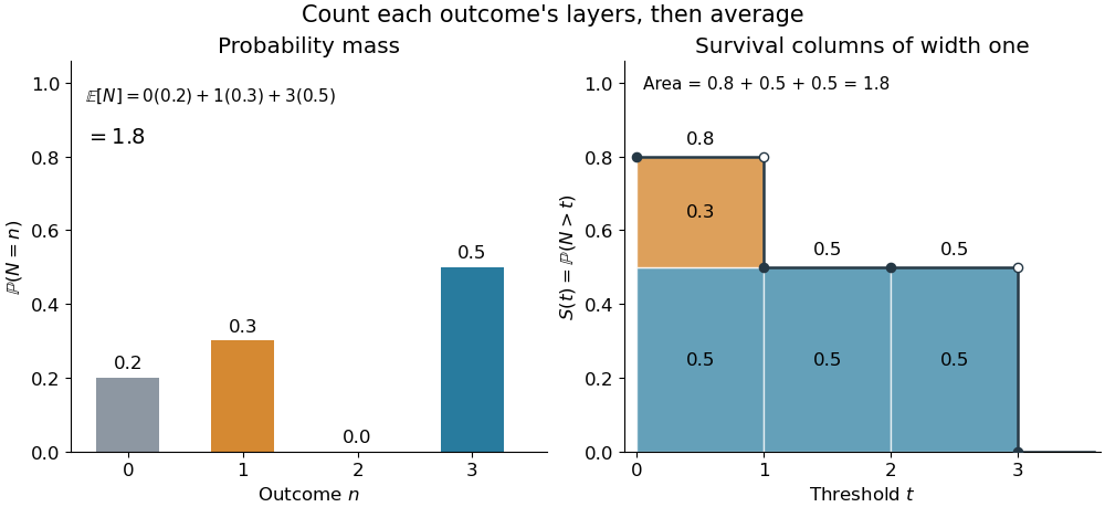
The same expected value from probability masses and survival columns
. The exact constructed probability mass function assigns to . The contribution appears in one survival column, while the contribution appears in three. Filled endpoints give the strict survival function at its jumps; open endpoints show the preceding height. The shaded area is . Details.
The indexing matters numerically. Starting the inclusive sum at zero adds , giving for this example. Starting the strict sum at one omits , giving . For a general nonnegative random variable, replacing with inside the integral is harmless: the difference is , nonzero at only a countable set of thresholds. For each positive integer , at most thresholds can have probability mass at least ; their countable union contains all thresholds with positive probability mass and has Lebesgue measure zero. This reasoning concerns an integral, not equality of the two survival function conventions at every point.
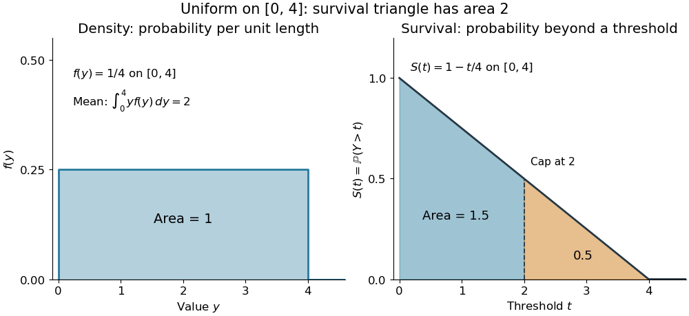
For a continuous original example, take the uniform distribution on the interval . Its survival function is for and zero for . The area is a triangle of base four and height one:Directly integrating against the probability density function gives the same expected value, . The integral of the probability density function alone is one; it is the survival function whose area is the expected value.

The proof counts layers of each outcome. For a realized value , the indicator function equals one over an interval of length , soTonelli theorem permits the interchange because the indicator function is nonnegative; no finite expected value is assumed. Similarly, an outcome contributes one indicator random variable for each of the events that occur:Again Tonelli theorem applies to the nonnegative sum, or equivalently the monotone convergence theorem applies to its partial sums. This exchanges counting layers within each outcome with averaging across outcomes. The existing integer-valued hypothesis in the tail-sum formula explains what changes when the values are not integers; the tail integral formula for moments weights the layers to obtain higher moments.
For an integrable random variable that can have either sign, apply the nonnegative formula separately to its positive part and negative part :Integrability makes both integrals finite. More generally the difference defines an extended expected value when at least one is finite; if both are infinite, subtraction does not define an expected value.[ref]
Random: Probability, Mathematical Statistics, Stochastic Processes by Kyle Siegrist. Expected Value, §2 Additional Properties, A General Definition: positive and negative parts and the condition on their expectations
Tail probabilities are often easier to measure or bound than a whole probability density function. For a device's survival time, the survival function records the probability of still operating at each threshold; its integral gives the mean operating time. A finite observation window naturally gives the expected value of a capped nonnegative random variable. For a mathematical bound, for all implies . The tail-sum formula turns control of a whole family of events into control of an average.
Indicator random variable Created 2026-09-24 Updated 2026-10-14
An indicator random variable is the indicator function of an event in a probability space: is one when occurs and zero otherwise. It has a Bernoulli distribution with parameter , so and . Even an event described without numbers becomes a numerical random variable in this way.
For a finite collection of events, their indicator random variables add up to the number that occur. Linearity of expectation therefore turns an average count into a sum of probabilities, without requiring independence. The fixed point count of a uniform random permutation provides an example where the indicators are dependent random variables.
Variance Created 2026-09-24 Updated 2026-10-14
The variance measures the mean squared distance of a random variable from its expected value. For a real square-integrable random variable ,The square prevents positive and negative deviations from cancelling. It also gives the variance squared units: if measures a length in metres, its variance has units of square metres. Its nonnegative square root is the standard deviation, which has the same units as .
For example, let take , and with equal probabilities. Its expected value is zero, but its variance is , and its standard deviation is . The constant random variable zero has the same expected value and zero variance: a mean alone does not describe the spread. The variance is zero exactly when almost surely.
The variance is useful because squared deviations interact neatly with linear combinations. The covariance supplies the cross terms when combining different random variables, and a covariance matrix organizes those terms for many variables. The characterization of variance as the minimum mean squared error of a constant also explains why the expected value is the best constant prediction under squared error.
Atmospheric spectral-feature amplitude Created 2026-09-24 Updated 2026-11-05
An exoplanet transmission spectrum measures a wavelength-dependent transit depth. In a simple opaque-disk geometry with uniform stellar brightness, an effective planetary radius gives , where is the stellar radius. If stronger atmospheric absorption increases that radius by , define as the atmospheric scale height and as the number of scale heights separating the two spectral levels. The additional occulted annulus givesThe last approximation requires . For instance, and give exact and leading estimate ; these are stipulated geometric ratios.
Since in the thin isothermal atmosphere model, larger temperature, smaller mean molecular weight or weaker gravity can increase the signal. The factor is set by the atmospheric opacity, composition and cloud structure; it is not a universal constant. Limb darkening, stellar heterogeneity and instrumental effects also affect the observed transit depth.[ref]
Theoretical Transmission Spectra During Extrasolar Giant Planet Transits by Sara Seager and Dimitar Sasselov. Transmission absorption through the atmospheric annulus; weak planet-to-star contrast and cloud sensitivity
Atmospheric escape Created 2026-09-24 Updated 2026-11-05
Atmospheric escape is the loss of gas from a planet to space. In Jeans escape, particles in the high-speed tail of a velocity distribution leave a nearly collisionless upper atmosphere if they exceed the local escape velocity. Hydrodynamic escape instead treats a collisional bulk outflow. Photochemical escape supplies another route by creating energetic reaction products.
Which description applies depends on gravity, heating, composition and the collision rate, rather than only on the planetary equilibrium temperature. Absorption of energetic stellar radiation can heat high atmospheric layers far above that temperature. Removing a light envelope changes the measured radius and future exoplanet atmosphere, connecting escape to the interpretation of a planetary mass-radius relation.
Exoplanet emission spectrum Created 2026-09-24 Updated 2026-11-05
An exoplanet emission spectrum describes the planetary thermal radiation as a function of wavelength. In an opaque exoplanet atmosphere, emerging light at a given wavelength comes predominantly from layers near outward optical depth of order one. Changing molecular opacity changes the layers sampled, so the spectrum jointly encodes composition and the atmospheric pressure-temperature profile.
A strong band is commonly darker when the sampled upper layers are cooler than the continuum-emitting layers. An atmospheric thermal inversion can instead put the band as an emission line. Occultation spectroscopy isolates the dayside spectrum, while exoplanet direct imaging can obtain it by spatially separating planetary and stellar light. A brightness temperature assigned to each band is a useful description of the data, but different bands can correspond to different physical layers.
Exoplanet transmission spectrum Created 2026-09-24 Updated 2026-11-05
An exoplanet transmission spectrum is the measured exoplanet transit depth as a function of wavelength. Light from the star passing through the limb of an exoplanet atmosphere is absorbed or scattered differently in different spectral bands. At a strongly absorbing wavelength, a ray becomes opaque farther from the centre, making the effective planetary radius larger.
The annulus model for transmission spectroscopy estimates the extra blocked area, while the slant optical depth of an isothermal atmosphere explains why this method can detect tenuous gas. Molecular-band amplitudes depend on the atmospheric scale height, abundances, and exoplanet cloud deck. Stellar contamination of a transmission spectrum and reference-pressure degeneracy in transmission spectroscopy limit how directly this observable can be translated into a unique composition.
Exoplanet secondary eclipse Created 2026-09-24 Updated 2026-11-05
An exoplanet secondary eclipse occurs when a planet passes behind its host star. Immediately outside the event the detector receives light from both bodies; during complete occultation it receives only stellar light. Their difference isolates planetary light, consisting of reflected stellar radiation, planetary thermal radiation, or both. Its fraction of the combined out-of-eclipse light is the eclipse depth.
Measuring that depth across wavelengths gives occultation spectroscopy of the visible dayside. The thermal eclipse depth connects a simple blackbody model to the radius ratio and brightness temperature. At visible wavelengths, reflected light can instead constrain geometric albedo. Changes in the host star or detector response must be modelled because the planetary signal is a small difference between two much brighter measurements.
Irradiated planetary atmosphere Created 2026-09-24 Updated 2026-11-05
An irradiated planetary atmosphere receives stellar radiation from above while intrinsic planetary heat flows outward from below. Stellar heating is therefore deposited where incident light is absorbed, rather than being supplied entirely at the bottom. Different opacities for stellar and planetary radiation can produce a deep, nearly isothermal region or an atmospheric thermal inversion.[ref]
On the radiative equilibrium of irradiated planetary atmospheres by Tristan Guillot. Abstract: simultaneous intrinsic and irradiation fluxes and distinct visible and thermal opacities
The absorbed power sets a global energy constraint, summarized by the planetary equilibrium temperature. The vertical atmospheric pressure-temperature profile additionally requires radiative transfer, convection and the heating depth. On a exoplanet under tidal locking, day-night heat redistribution also matters because only one hemisphere receives direct starlight.
First excited state Created 2026-09-24 Updated 2026-11-05
A first excited state has the lowest allowed energy eigenvalue strictly above the ground-state energy, when such a next eigenvalue exists. The level can be degenerate, in which case several independent first excited states share that energy.
For a quantum harmonic oscillator, the ground state has occupation and the first excited state , separated by . In an infinite square well labeled by , the first excited state instead has label . “First” orders the energies rather than imposing a universal index convention. A system with a continuum starting at its lowest energy need not possess a normalizable first excited state at all.
Level repulsion in a two-level Hamiltonian Created 2026-09-24 Updated 2026-11-05
There are unlisted articles, also show them or only show them.