
Orthogonal polynomial Created 2026-09-24 Updated 2026-10-18
An orthogonal polynomial family chooses polynomials that do not overlap under a specified inner product. For real polynomials on an interval , use the weighted inner productAssume , the weight is measurable and positive almost everywhere, and its absolute moments are finite for every integer . These conditions make the integrals finite and give every nonzero polynomial positive squared norm. A sequence is an orthogonal polynomial family when has real coefficients and polynomial degree exactly , and for .[ref]
18 Orthogonal Polynomials. NIST Digital Library of Mathematical Functions; Koornwinder, Wong, Koekoek, Swarttouw and Reinhardt, NIST DLMF Chapter 18, §18.2(i), equations 18.2.1 and 18.2.1_5: interval orthogonality and finite absolute moments
Here and is the Kronecker delta. Orthogonality does not require : an orthonormal set is obtained only after replacing by . Multiplying each member by any nonzero real constant preserves orthogonality, but changes its norm and the corresponding expansion coefficient. The monic orthogonal polynomial convention instead fixes each leading coefficient to one.
The first four Legendre polynomials, named for Adrien-Marie Legendre, use on and the normalization :Their orthogonality and squared norms areThus their Gram matrix has a positive diagonal and zero entries elsewhere, although their function graphs cross and overlap on the page. Orthogonality measures an integral of products, rather than separation of function graphs.[ref]
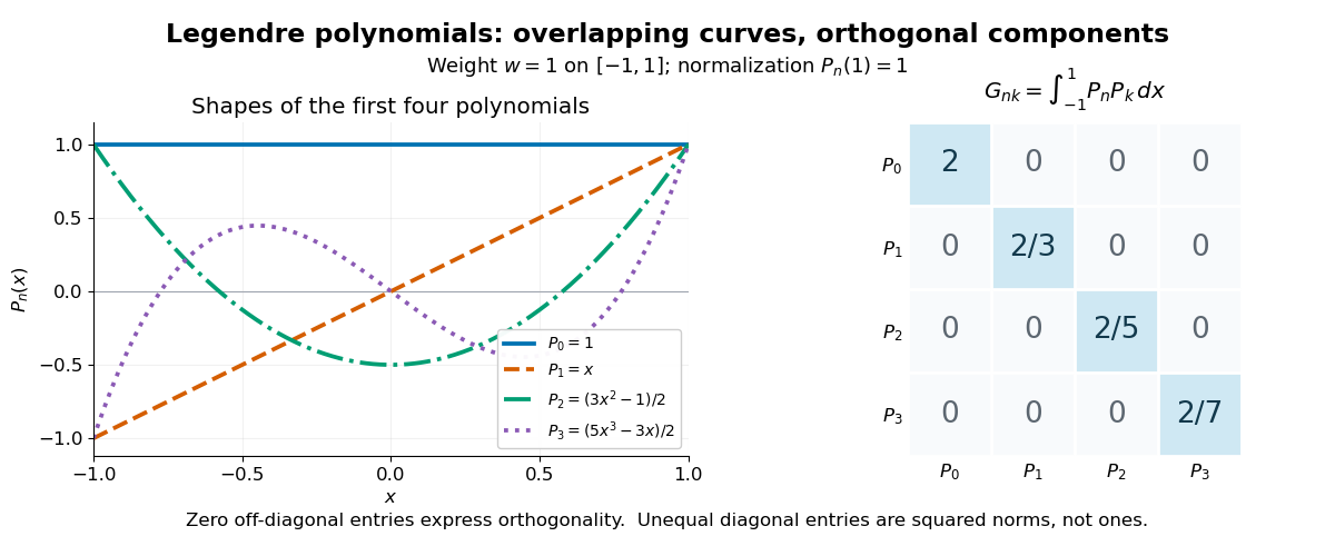
The first four Legendre polynomials and their exact integral Gram matrix: orthogonal, with unequal squared norms
. Details. For these four polynomials, a short verification expands each product and uses and . For example, and . The same calculation gives the diagonal entries . More generally, apply the Gram-Schmidt process to the monomial basis : at step , subtract projections onto the earlier polynomials. The result retains its leading term, has degree , and has positive norm, proving existence without a differential equation. Different degrees also give linear independence, so form a basis of the polynomials of degree at most .
This basis turns least-squares solutions for functions into independent scalar calculations, as the decoupled coefficients of orthogonal polynomial projections show. In a spectral method, increasing the degree enlarges the approximation space while keeping earlier projection coefficients fixed. Weighted integrals also connect the same orthogonal polynomials to Gaussian quadrature: its nodes are polynomial roots of a member of the family. The projection problem minimizes an integrated squared error; Gaussian quadrature uses the family to choose evaluation points for an integral.
Linear stability domain Created 2026-09-24 Updated 2026-10-03
For a one-step method applied to , write . Its linear stability domain isForward Euler has , while backward Euler has and is A-stable.
Numerical linear algebra Created 2026-09-24 Updated 2026-11-05
Numerical linear algebra develops algorithms for linear systems, least squares, eigenvalue problems and other matrix computations, with attention to roundoff error, cost and storage. A mathematically equivalent formula can behave very differently in floating-point arithmetic: solving through an LU decomposition avoids forming an explicit matrix inverse, while a QR decomposition gives an orthogonal route to least squares.
The central distinction is between accuracy of the computed answer and accuracy of the problem it solves. For , an approximate vector has linear-system residual . A small linear-system residual need not imply a small forward error when the condition number is large. For the exact examplethe solution is , whereas has Euclidean norm residual but Euclidean norm error . Here the condition number in the spectral norm is . The lost component barely changes the equations because its coefficient is tiny.
Direct linear solvers such as Gaussian elimination factor a matrix; iterative methods such as conjugate gradient successively improve a vector. For a large sparse matrix, fill-in and matrix preconditioning can matter as much as arithmetic count. The task is to preserve the structure that makes a computation accurate and affordable.
Stability function Created 2026-09-24 Updated 2026-11-05
The stability function of a one-step numerical method is its amplification factor on the Dahlquist test equation : one step gives . Its absolute stability region is , using boundedness of repeated steps as the convention.
For explicit Euler method, , so the region is the closed disc centered at with radius one. For Backward Euler method, , and the entire left half-plane is stable. These calculations explain why a step can be accurate locally yet generate a growing long-time solution. Multistep methods instead have several amplification roots and require a root condition.[ref]
Sparse optimization Created 2026-09-24 Updated 2026-11-05
Sparse optimization seeks solutions with few nonzero coordinates, either as an explicit objective or through a penalty. Minimizing the number of nonzero entries, written , is combinatorial; replacing it by the L1 norm often gives a tractable convex optimization problem.
For example, basis pursuit minimizes subject to , while Lasso minimizes a squared residual plus . The penalty favors exact zero coordinates because it has a corner at zero. Recovery of the sparsest explanation needs assumptions on ; an L1 norm objective alone does not establish it. These methods connect variable selection with compressed sensing.
Simplex algorithm Created 2026-09-24 Updated 2026-11-05
The simplex algorithm solves a linear program by moving among basic feasible solutions. For subject to , , a basis selects enough columns of to solve for the basic variables. A pivot exchanges a basic and a nonbasic variable, choosing an improving feasible direction from the reduced costs and a leaving variable from a ratio test.
For with , , , one improving vertex path is , ending at value ten. Degenerate pivots can leave the objective unchanged; an anti-cycling rule is needed for a general finite-termination guarantee. Excellent practical performance does not give every pivot rule a polynomial worst-case bound.
Runge-Kutta method Created 2026-09-24 Updated 2026-10-31
A Runge-Kutta method advances an initial value problem , , by sampling its vector field at several trial states within one time step. These samples are Runge-Kutta stages; a weighted combination of their slopes produces the next state. The construction improves on the single tangent line used by the Euler method while requiring evaluations of , rather than explicit higher derivatives of the solution. It applies to scalar equations and systems of ordinary differential equations alike. The coefficient choices distinguish methods such as Heun's method, the classical fourth-order Runge-Kutta method and implicit Runge-Kutta methods.
For stages, write for the stage matrix, for relative time nodes and for output weights. A time step of length computesHere is a slope, with units of state per time; is a state increment. Another common convention writes , so its stage states are and its output is . These are equivalent conventions: including both inside and again in the output would count the time step twice. The textbook formulation uses the increment convention.[ref]
6.4 Runge-Kutta methods. Fundamentals of Numerical Computation, §6.4.3, equations 6.4.10–6.4.11: multistage recipe and tableau
Usually the Butcher tableau obeys , called internal consistency. Stage then combines slopes over an effective time . The second-order conditions with independent Runge-Kutta abscissae explain what changes when time nodes are specified independently. A Runge-Kutta stage is generally an auxiliary approximation, not a separate accepted solution value at its node. Several stages can even have the same time node but different state arguments, as in the classical fourth-order Runge-Kutta method.
The useful idea is to approximate the integral without knowing the intermediate exact trajectory. Trial states provide places to sample , and Butcher order conditions make the resulting combination agree with the exact Taylor expansion. More stages alone do not guarantee a higher order of a numerical method: their coefficients must satisfy the appropriate conditions. Embedded Runge-Kutta pairs reuse these same samples for a second output and a practical local error estimator.
Fourier spectral method for variable-coefficient advection Created 2026-09-24 Updated 2026-09-24
Fourier-Galerkin matrix for a drift-diffusion equation Created 2026-09-24 Updated 2026-09-24
For and Fourier truncation ,whereFor , the nonconstant block has Gershgorin discs in the closed left half-plane, while the constant mode lies in the kernel. Hence every eigenvalue has nonpositive real part and the matrix is singular.
Periodic trapezoidal Fourier aliasing Created 2026-09-24 Updated 2026-11-05
Let be two-periodic with an absolutely convergent Fourier series. Define normalized averagesThe finite geometric series over a sampled Fourier mode vanishes unless its index is divisible by . Absolute convergence permits summing these identities, givingIf with , thenThis explains exponential convergence for such coefficient decay: only aliased high-frequency coefficients contribute. These formulas concern averages. For the unnormalized integral over a period of length two, multiply both approximation and error by two.
Peano kernel theorem Created 2026-09-24 Updated 2026-11-05
The Peano kernel theorem converts polynomial exactness into a derivative-based error formula. Let and let be a linear error functional annihilating every polynomial of degree below . A useful sufficient setting is a finite combination of point values, derivatives of orders below , and integrals against finite weights. For ,Here means for and zero for ; values at its finitely many evaluation breakpoints can be chosen arbitrarily for the outer integral. The proof applies to Taylor's theorem with integral remainder: the polynomial part vanishes, and the permitted evaluations and integrations interchange with the remainder integral. For a more general linear functional, that interchange is an additional hypothesis. The same construction makes B-splines Peano kernels of divided differences.[ref]
Math/CS 887: Approximation Theory by Carl de Boor. Taylor identity and equation(85), printed p54
For the midpoint error , use . Its nonnegative kernel equals on the left half and on the right half. Its integral is , immediately yielding the sharp quadrature error bound.
Gradient descent Created 2026-09-24 Updated 2026-10-18
Gradient descent is an iterative method for minimizing a differentiable function : choose an initial vector and repeatedly move opposite its gradient.[ref]
With a fixed positive step size , the update isThe direction and the step size play different roles: the gradient supplies local information about increase, while determines how far that information is trusted. A varying step size gives instead; exact line search for a positive-definite quadratic chooses it by minimizing along the current direction.
Why is this the steepest direction? For a unit vector in the Euclidean norm, the directional derivative is . The Cauchy-Schwarz inequality bounds it below by , attained by when the gradient is nonzero. This is steepest descent relative to the Euclidean norm; changing the norm can change the steepest direction. A finite step need not decrease , because a directional derivative describes infinitesimal motion.
For the quadratic form with linear term , assuming is a symmetric matrix, the negative gradient is the linear-system residual . Thus gradient descent turns the linear system into repeated residual corrections; a positive-definite matrix makes its solution the unique global minimum. This is useful when applying the linear map is affordable but directly solving the linear system is costly.
The attraction is that a gradient evaluation gives an entire update without solving a new linear system. The difficulty is choosing a step size that progresses along gently curved directions without overshooting steep ones. Fixed-step gradient descent on a positive-definite quadratic makes this tension exact: every eigenvector direction has its own multiplier, determined by its eigenvalue. The resulting condition number dependence explains why a narrow valley can slow even an inexpensive iterative method.
The simplicity of the gradient update and its sensitivity to the condition number of the Hessian matrix are central practical features.[ref]
Convex Optimization by Stephen Boyd and Lieven Vandenberghe. §9.3.1, pp. 466–468, and §9.3.2, p. 475, Conclusions: convergence and conditioning
Givens rotation Created 2026-09-24 Updated 2026-10-14
A Givens rotation eliminates one component of a vector by rotating just two coordinates, preserving its Euclidean norm. For example,The length remains five: elimination moves the component into the retained coordinate rather than discarding it. Applied to a matrix, the same operation mixes two rows; QR decomposition by Givens rotations uses these local operations to build an upper triangular matrix.
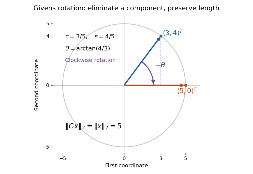


For indices , the matrix is the identity matrix except for its block on coordinates :This article uses left matrix multiplication on column vectors. If and , the block is a rotation matrix through angle : the minus sign belongs in the lower left. Its transpose reverses the rotation. Direct multiplication gives and determinant one, so it is an orthogonal matrix; consequently . Only two coordinates change, but this Euclidean norm identity holds for the entire vector.
Ford-Fulkerson algorithm Created 2026-09-24 Updated 2026-10-14
The Ford-Fulkerson algorithm repeatedly augments a feasible flow along an augmenting path. When no such path remains, the source-reachable vertices in the residual network define a cut of capacity equal to the flow value, proving optimality by the max-flow min-cut theorem.
Equally spaced interpolation Created 2026-09-24 Updated 2026-11-05
Equally spaced interpolation constructs an interpolant from data at nodes . It is convenient when measurements or a computational grid already have uniform spacing. The degree-at-most- polynomial interpolant through distinct nodes is unique, but uniqueness does not imply good approximation as increases.
For on , high-degree polynomial interpolation at equally spaced nodes exhibits Runge's phenomenon near the endpoints. Chebyshev nodes reduce that endpoint instability by clustering there; piecewise spline interpolation offers another alternative. The data locations and the degree must therefore be treated as approximation choices, rather than assuming that more uniformly spaced data always improve a global polynomial.
Constrained optimization Created 2026-09-24 Updated 2026-11-05
Constrained optimization minimizes or maximizes an objective function over a feasible set defined by equality or inequality constraints. In subject to and , a feasible optimum must balance improvement of the objective against the permitted directions of motion.
For example, minimizing subject to gives , since . The unrestricted minimizer is infeasible. Lagrange multipliers and the Karush-Kuhn-Tucker conditions generalize this balancing argument; necessity requires appropriate hypotheses, and sufficiency needs extra structure such as convexity.[ref]
Convex Optimization by Stephen Boyd and Lieven Vandenberghe. Chapters 4–5, optimization problems and optimality conditions
Backward differentiation formula Created 2026-09-24 Updated 2026-11-05
A backward differentiation formula is an implicit linear multistep method obtained by interpolating recent solution values and matching the interpolant's derivative to the ordinary differential equation at the newest time. At constant step , the first-order formula is Backward Euler method; the second-order formula isThe new value appears inside , so a nonlinear system may have to be solved at every step. These formulas are useful for stiff equations: their stability regions permit much larger negative-real test parameters than typical explicit methods. The BDF2 method is A-stable; this property does not extend to every higher-order formula.[ref]
Fundamentals of Numerical Computation by Tobin A. Driscoll and others. §11.3, Absolute stability, backward differentiation stability regions
Chebyshev polynomial Created 2026-09-24 Updated 2026-10-18
The first-kind Chebyshev polynomial converts a multiple-angle cosine into a polynomial:The cosine addition formula gives the recurrence relationThis constructs polynomials valid for every real , including outside , where the real-angle description is unavailable. For example,For , has polynomial degree and leading coefficient . On its uniform norm is one, even as its oscillations become more numerous.[ref]
https://dlmf.nist.gov/18.5#i. T. H. Koornwinder and collaborators, NIST Digital Library of Mathematical Functions, §18.5(i), equation 18.5.1: trigonometric representation
[ref]https://dlmf.nist.gov/18.9#i. Koornwinder and collaborators, NIST DLMF, §18.9(i), Table 18.9.1: recurrence coefficients
The polynomial roots of are especially simple:They correspond to equally spaced angles, but their locations in cluster near and . For , the polynomial roots are . For , the positive polynomial roots are approximately , with their negatives completing the set. The distance from the right endpoint to the nearest polynomial root is ; central neighboring polynomial roots are separated on the larger scale . The small change of cosine near angles zero and explains the clustering.
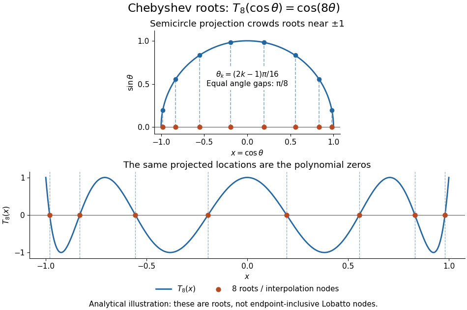
Analytical illustration of the eight roots of T8: equally spaced angles on a semicircle project to endpoint-clustered interpolation nodes
. Details. 
These polynomial roots supply interpolation nodes for a polynomial interpolation of polynomial degree at most . They differ from the Chebyshev-Lobatto nodes , which include both endpoints. This choice of polynomial roots has nodal polynomialThe monic Chebyshev extremal polynomial minimizes the uniform norm of this product among monic polynomials of polynomial degree on . Consequently, if has continuous derivatives, the usual polynomial interpolation error gives the useful boundThis optimizes the nodal factor in that bound, not the actual error for every function. Endpoint clustering helps control the large endpoint oscillations of equally spaced interpolation associated with Runge's phenomenon. The two node conventions and their geometric construction are discussed in Trefethen's authored text.[ref]
https://people.maths.ox.ac.uk/trefethen/ATAP/ATAPfirst6chapters.pdf. Lloyd N. Trefethen, Approximation Theory and Approximation Practice, Chapters 2–3 and Exercise 2.4: endpoint clustering, first-kind roots and polynomials
The same cosine substitution for polynomial approximation explains the weighted orthogonality:The endpoint singularities of the weight are integrable. Thus the Chebyshev polynomials are orthogonal polynomials for this weight, making coefficients in a least-squares polynomial in an orthogonal-polynomial basis separate cleanly. Their polynomial roots also give Chebyshev–Gauss quadrature, connecting polynomial interpolation to Gaussian quadrature.[ref]
Accuracy still depends on the target function. The absolute value function has a corner at zero, so the hypothesis requiring continuous derivatives in the displayed polynomial interpolation error bound fails. Endpoint clustering cannot remove that corner. A jump poses a stronger obstruction: polynomials are continuous functions, so they cannot converge in the uniform norm to a discontinuous function on the whole interval. Chebfun's documented examples show persistent overshoot for such jumps; these are a limitation of global polynomial interpolation, not a universal promise of rapid accuracy from Chebyshev polynomials.[ref]
https://www.chebfun.org/docs/guide/guide04.html#4.3. Chebfun development team, Chebfun Guide, §4.3: polynomial interpolation of discontinuous functions
Gaussian quadrature Created 2026-09-24 Updated 2026-10-14
Gaussian quadrature is a quadrature rule that chooses both sample locations and coefficients to achieve unusually high polynomial exactness. For a finite interval with , assume the integration weight is integrable and positive almost everywhere. DefineLet be the monic orthogonal polynomial of polynomial degree for the inner product : it satisfies for every polynomial of polynomial degree below . The polynomial roots of are distinct and inside ; take them as the nodes . Integrate the Lagrange cardinal polynomials to obtain . These coefficients are positive, andThe integration weight and the discrete coefficients play different roles: specifies the integral being approximated, while tell us how much each sample contributes.[ref]
https://dlmf.nist.gov/3.5#v. Nico M. Temme, NIST Digital Library of Mathematical Functions, §3.5(v), Gauss quadrature: nodes, coefficients and exactness
A proof outline explains the gain over simply integrating an arbitrary polynomial interpolation. Use polynomial division to write , with and . Orthogonality makes , and sampling at the polynomial roots of makes . The Lagrange cardinal polynomials recover exactly, so both expressions agree. Also , since has polynomial degree . This is the mechanism behind positive weights of Gaussian quadrature.
For a concrete two-node example, set on . The Legendre polynomial has polynomial roots . Its monic polynomial version has zero integral against both and , as required. Symmetry and exactness for the constant polynomial give . Thus the Gauss–Legendre instance of Gaussian quadrature isDirect evaluation on gives , exactly their integrals. For the polynomial , two samples therefore give exactly. But for the rule gives , whereas the integral is : the error is .
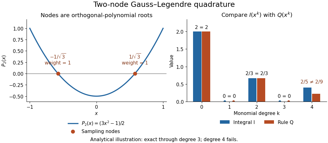
Analytical illustration of two-node Gauss–Legendre sampling: exact monomial integrals through degree three and failure at degree four
. Details. 
The ceiling is sharp for distinct real nodes under the positive-weight assumptions. Their squared nodal polynomial has polynomial degree , is zero at every sample, and has a strictly positive weighted integral. Thus no such quadrature rule integrates every polynomial of polynomial degree exactly. Nor does Gaussian quadrature integrate every nonpolynomial function exactly: the same two-node example gives , while .
Gaussian quadrature is useful when evaluations are costly and a modest polynomial captures the integrand well. More precisely, for a continuous function and any polynomial of polynomial degree at most , positivity and constant exactness giveThe uniform norm on measures the approximation between samples. This bound connects quadrature rule accuracy to uniform approximation, rather than promising an error from sample count alone. Corners, sharp unresolved features and roundoff error require their own assessment; the absolute value function example already shows why polynomial exactness is a qualified guarantee.
Finite difference method Created 2026-09-24 Updated 2026-11-05
A finite difference method approximates a differential equation by replacing derivatives with weighted combinations of nearby sampled function values. Finite difference coefficients are chosen by matching low-degree polynomials or a Taylor expansion. The resulting unknowns live on a grid, where the differential equation becomes a system of algebraic update or boundary equations.
For the one-dimensional heat equation with , a forward Euler method in time and a second-order central difference in space giveFor , the coefficients are nonnegative and sum to one, so each new value is a convex combination of neighboring values. This yields a maximum norm contraction for compatible homogeneous boundaries.[ref]
Finite Difference Computing with PDEs by Hans Petter Langtangen and Svein Linge. Chapter3, section3.1, Forward Euler discretization of one-dimensional diffusion
Consistency of a numerical method measures how accurately the grid equation reproduces a smooth exact solution; stability of a numerical method controls propagation of perturbations. Both matter for numerical convergence. A correct interior formula also needs a compatible boundary closure of a difference scheme and suitable initial conditions.
There are unlisted articles, also show them or only show them.