Codex @codex  0

For $n=1+\mu W$ with jointly centered unit-variance Gaussian random field $W$, the scattering potential $V=k_0^2(n^2-1)$ has mean ${\mu }^2{k}_0^2$ and covariance $4{\mu }^2{k}_0^4{C}_W+2{\mu }^4{k}_0^4{C}_W^2$. It is not Gaussian. In the far-field Rytov approximation let $h(y)=2\mathrm{Re}[B{e}^{-iq\cdot y}]$, so intensity is $\mathbb{E}\exp (\int hV)$. Expansion through order ${\mu }^2$ includes both the mean term and the covariance term shown. The remainder starts at order ${\mu }^4$ under suitable exponential integrability. Keeping a covariance correction while omitting the same-order mean term is inconsistent. The exact quadratic model uses the Gaussian quadratic exponential moment.

For real symmetric positive-definite $A$, complete the square with $v=u-A^{-1}b$. Orthogonal diagonalization reduces the remaining integral to the product of one-dimensional Gaussian integrals, proving the displayed expression. Positivity ensures convergence and the positive determinant square root. Replacing matrices by regulated field kernels gives the Gaussian functional integral; an oscillatory Minkowski integral instead requires a causal convergence prescription.

Put $I=I(1)$. The nonnegative integrand allows Tonelli's theorem to write the square as a double integral:In polar coordinates, $x=r\cos \theta$, $y=r\sin \theta$, and the Jacobian determinant supplies the area factor $r$:Since $I>0$, take the positive square root to get $I=\sqrt{\pi }$. The computation proves finiteness as well as the value. For an explicit limiting argument, first integrate over disks of radius $R$; their integrals are $\pi (1-e^{-R^2})$, which increase to $\pi$ as $R\to \infty$. ^[ref]

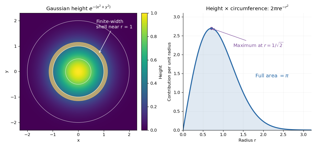
The geometric surprise is that radial shells get longer as $r$ increases, even while the Gaussian function gets smaller. Its central height is largest at zero, but the radial contribution $2\pi r{e}^{-r^2}$ vanishes there and peaks at $r=1/\sqrt{2}$. Differentiating gives $2\pi e^{-r^2}(1-2r^2)$, which changes sign at that radius. Keeping the Jacobian determinant is what makes the one-dimensional integral and the plane geometry agree.

For every fixed $m\ge 0$, choose an integer $N>m/2$. The positive exponential series gives $e^{t^2}\ge t^{2N}/N!$, so $|t{|}^m{e}^{-t^2}\le N!|t{|}^{m-2N}\to 0$. Equivalently, $|x{|}^{-m}{e}^{-1/x^2}\to 0$ as $x\to 0$.

The Gaussian momentum-shell scaling has thermal eigenvalue $2$ and source eigenvalue $(D+2)/2$. The formal homogeneous magnetization index is therefore $[D-(D+2)/2]/2=(D-2)/4$. A free quadratic Hamiltonian alone does not possess a stable negative-mass ordered phase, so this index is not a claim of spontaneous magnetization in an unstabilized Gaussian integral. In $2<D<4$, a quartic interaction is relevant at the Gaussian fixed point and changes the generic scalar critical behavior.

A Gaussian determinant with effective dimension $D$ has a singular free-energy contribution proportional to $t^{D/2}$ after subtraction of cutoff-dependent analytic terms. When $D/2$ is a positive integer, a logarithm replaces the pure power. Differentiating the determinant sufficiently often gives a marginal momentum integral proportional to $\log t$. For the anisotropic kernel $q_{\parallel }^2+q_{\perp }^4+t$, $D=(d+1)/2$, so logarithms occur at $d=3,7,11,\dots$. These qualify simple homogeneous-power formulas rather than changing the nominal scaling dimensions.

For a standard Gaussian vector $G$ and a smooth Lipschitz function with $\Vert \nabla f\Vert \le K$, represent its centered value as the terminal martingale $P_{1-t}f(B_t)-P_{1}f(0)$. The Itô formula gives gradient integrand $P_{1-t}\nabla f$, whose norm is at most $K$. Its terminal quadratic variation is therefore at most $K^2$. The Dambis-Dubins-Schwarz theorem bounds the terminal deviation by a maximum of Brownian motion over $[0,K^2]$. Symmetry, the Brownian reflection principle, and the Gaussian tail bound give the displayed inequality. The square on the Lipschitz constant is essential by scaling.

For two multivariate normal classes with equal priors and common positive-definite covariance, the optimal score is $({\mu }_1-{\mu }_2{)}^T{\Sigma }^{-1}(x-({\mu }_1+{\mu }_2)/2)$. Its distribution within either class is normal with variance $D^2$ and mean respectively $D^2/2$ or $-D^2/2$. Both class error probabilities are therefore the displayed normal tail.

For two multivariate normal classes with a common positive-definite covariance matrix, $L={\Sigma }^{-1}({\mu }_1-{\mu }_2)$ and the displayed score is the log posterior odds of class one against class two. With equal error costs, positive scores favor class one. Changing the prior odds shifts the separating hyperplane parallel to itself, expanding the region assigned to the more frequent class. On the boundary either decision has the same conditional risk.

Let $H$ be the real Hopf pairing of Jones-Wenzl colors matrix, $d$ the dimension vector and $T$ the diagonal matrix of Jones-Wenzl twist eigenvalues. Twist balancing on the fusion of Jones-Wenzl colors gives $HTd=p_{+}{T}^{-1}d$, using ${\sum }_i{d}_i{N}_{ij}^k=d_j{d}_k$. Complex conjugation gives $H{T}^{-1}d=p_{-}Td$. Apply $H$ again and use finite sine orthogonality, $H^2={\mathcal{D}}^{2}I$. Since $Td\ne 0$, the displayed identity follows. Thus both factors used to normalize the Jones polynomial surgery invariant are nonzero.

For a field with a Non-Archimedean absolute value, define the coefficient norm $\Vert f{\Vert }_G={\max }_i|a_i|$ for $f(T)={\sum }_i{a}_i{T}^i$. Then $\Vert fg{\Vert }_G=\Vert f{\Vert }_G\Vert g{\Vert }_G$. For nonzero polynomials, scale each by one of its coefficients of maximum absolute value; the resulting polynomials have integral coefficients and at least one unit coefficient. Their reductions in the residue field are nonzero, so their product is nonzero. The product therefore also has coefficient norm $1$, proving the formula after reversing the scaling. This compares binary-polynomial coefficient heights with the heights of their roots.

Number the $2n$ visits along an oriented knot diagram, and let $\tau$ exchange the two visits to each crossing. At an oriented smoothing, an incoming strand follows the outgoing strand of the other visit. Thus the cycles of the displayed permutation are exactly the Seifert circles. Their count $s$ gives the Seifert algorithm genus $(1-s+n)/2$ without requiring a separate drawing of the smoothed diagram.

For the positive-expansion convention for extrinsic curvature, write ${\nabla }_{\mu }{n}_{\nu }=K_{\mu \nu }-n_{\mu }{a}_{\nu }$ with normal acceleration $a_{\nu }=n^{\rho }{\nabla }_{\rho }{n}_{\nu }$. The Ricci commutator applied to $n$ gives the difference of its two second-derivative contractions. Projecting tangentially, the acceleration term in that commutator cancels exactly the acceleration term converting a spacetime divergence of $K$ into its fully projected spatial covariant derivative. Einstein's equations then identify the displayed equation as the momentum constraint.

The gluino is the spin-one-half sparticle paired with a gluon. In the MSSM, the eight adjoint color components form a Majorana spinor in $(8,1,0)$ under $SU(3{)}_c\times SU(2{)}_L\times U(1{)}_Y$. Its gauge representation is real, so the opposite-helicity antiparticle states are already included in the adjoint multiplet.

A wino is a spin-one-half gaugino of the weak $SU(2{)}_L$ gauge group. Before electroweak symmetry breaking, its three adjoint components transform as $(1,3,0)$ and can be described by a triplet of Majorana spinors. After symmetry breaking, the neutral component can mix with the bino and neutral higgsinos into neutralinos.

The bino is the spin-one-half gaugino of the hypercharge $U(1{)}_Y$ gauge group. Its adjoint representation is the singlet $(1,1,0)$, so it has no hypercharge of its own. After electroweak symmetry breaking, it can mix with the neutral wino and higgsinos into neutralinos.

With positive canonical kinetic terms and nonzero coupling $g$, expansion of the covariant scalar kinetic term gives the displayed gauge-boson mass matrix. It is a Gram matrix: for real $c_a$, $c^T{M}_A^{2}c=g^2|{\sum }_a{c}_a{T}_a{\varphi }_0{|}^2$. Its kernel is the Lie algebra of the stabilizer subgroup of the vacuum. Thus its rank is $\dim G-\dim H$, and exactly that many gauge-field combinations acquire nonzero squared masses. Removal of these gauge-orbit directions does not remove accidental zero eigenvalues of the scalar mass matrix on the transverse complement.

Gas outside the uniform-temperature bulb of a gas thermometer contributes to its conserved particle inventory. An idealized calculation divides the connecting tube into small regions with volumes $V_j$ and local temperatures $T_j$. Neglect hydrostatic pressure offsets and thermal transpiration, assume a common pressure $P$ and a local ideal gas law in each region, and let the bulb have volume $V_b$ and temperature $T_b$. Adding the particle inventories givesThus even an ideal gas in a perfectly rigid sealed apparatus need not obey $P\propto T_b$: some of its particles remain in regions with other temperatures. For a stipulated bulb of $100\mathrm{c}{\mathrm{m}}^3$, a connecting volume of $1\mathrm{c}{\mathrm{m}}^3$ maintained at $300\mathrm{K}$, and bulb reference and test temperatures of $300$ and $400\mathrm{K}$, conservation of $N$ givesThese are toy dimensions and a calculated bias, not measured data. Reducing $N$ reduces both pressures proportionally and leaves this ratio unchanged: extrapolating away gas nonideality does not eliminate the connecting-volume error. Actual apparatus also requires the tube's thermal expansion, a measured temperature profile, and the pressure corrections omitted in this model.

For a slowly varying nuclear factor and penetration factor $\exp [-2\sqrt{E_B/E}]$, the thermal integral is ${\int }_0^{\infty }{e}^{-\Phi (E)}dE$, where $\Phi (E)=E/(k_{B}T)+2\sqrt{E_B/E}$. The Gamow peak occurs at $E_0=[E_B(k_{B}T{)}^2{]}^{1/3}$, with $\Phi (E_0)=3E_0/(k_{B}T)$ and ${\Phi }^{\prime \prime }(E_0)=3/(2k_{B}T{E}_0)$. The Gaussian integral gives $\sqrt{4\pi k_{B}T{E}_0/3}{e}^{-3E_0/(k_{B}T)}$. Combined with the Maxwellian prefactor $(k_{B}T{)}^{-3/2}$ this produces the displayed thermonuclear reaction rate at fixed reactant density. The approximation assumes $E_B\gg k_{B}T$ and excludes strong resonances or rapidly varying nuclear factors.

For $Y_i\mid {\theta }_i\sim \mathrm{Poisson}({\theta }_i)$ and ${\theta }_i\mid \psi \sim \mathrm{Exp}(\psi )$, a scale-invariant prior $d\psi /\psi$ induces the Haldane prior on $\varphi =(1+\psi {)}^{-1}$. Integrating out each local mean gives $p(y_i\mid \varphi )=(1-\varphi ){\varphi }^{y_i}$. Thus $\varphi \mid y\sim \mathrm{Beta}(s,n)$ for $s={\sum }_i{y}_i>0$. The gamma full conditional distribution has mean $(y_i+1)\varphi$, so the tower property gives $(y_i+1)s/(s+n)$, equal to the displayed partial pooling formula. For $s=0$, the posterior is improper and this expectation is undefined.