
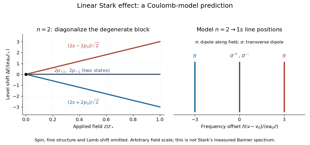
For an illustrative emission calculation, retain only the first-order shifts above and neglect the quadratic shift of the hydrogen atom ground state. The unperturbed Lyman-alpha line frequency is . The possible offsets areThe outer pair originates in the parts of and has transition electric dipole moments along the applied electric field, conventionally called components. The central pair originates in and has transverse rotating transition electric dipole moments, conventionally called components. Because electromagnetic radiation is transverse, the components disappear when viewed along the electric field. Viewed from the side, the and components have polarization of an electromagnetic wave respectively parallel and perpendicular to the applied electric field. Line intensities additionally require the initial quantum state populations and the collection geometry.

Onsager reciprocal relation Created 2026-10-18 Updated 2026-11-05
An Onsager reciprocal relation connects cross-couplings between near-equilibrium transport processes. Choose thermodynamic forces and fluxes so that their products give the entropy production, and write . With microscopic reversibility, no imposed time-reversal-breaking field and variables with the appropriate matching time-reversal parity, the coefficients obey . The choice of conjugate force and flux matters: arbitrary rescaling of just one coefficient need not preserve its numerical symmetry.
For coupled thermal and electrical transport, a thermal driving force can induce charge flow while an electrical driving force induces heat flow. Reciprocity relates those cross effects, reducing the number of independent transport measurements. Lars Onsager's 1931 paper develops this reasoning from microscopic reversibility and distinguishes it from thermodynamic positivity alone.[ref]
Reciprocal Relations in Irreversible Processes. I. by Lars Onsager. Abstract and §§1–3: coupled irreversible processes; reciprocal relation supplies information beyond thermodynamics
External magnetic fields and odd time-reversal variables require a generalized parity-sensitive relation rather than an unconditional symmetric matrix. Kramers-Kronig relations 2026-10-18
Causality constrains the real and imaginary parts of a frequency-dependent linear response. For a dielectric with at large frequency, the convention givesThe integral is a Cauchy principal value. Absorption and optical dispersion therefore cannot be specified independently.
Zero-frequency cancellation of a causal response kernel Created 2026-10-18 Updated 2026-10-20
For an integrable linear response kernel and input , the convolution theorem gives . The integrated output is therefore zero for every integrable input if and only if . For a sum of causal damped sines, , the condition is . If all are positive, nonzero terms of both signs are needed; a term with vanishes identically.
Kundt's tube 2026-10-18
A Kundt's tube turns an invisible standing wave into a measurable spatial pattern. A driven air column supports a longitudinal wave; measuring its frequency and the spacing of repeated nodes of a standing wave gives the speed of sound. The same drive can compare the wavelengths in a gas and a vibrating solid. August Kundt's 1866 paper introduced acoustic dust figures; its footnote explicitly counts successive nodes of a standing wave as half a wavelength.[ref]
Ueber eine neue Art akustischer Staubfiguren und über die Anwendung derselben zur Bestimmung der Schallgeschwindigkeit in festen Körpern und Gasen by August Kundt. 1866 publisher record; original p. 502 footnote on half-wavelength spacing
The attractive feature is the separation of measurements: a clock or frequency counter measures repetition in time, while a ruler measures repetition in space. Their product supplies a propagation speed. The pressure pattern and the fluid-motion pattern are different, however; identifying which one a detector responds to prevents a quarter-wavelength mistake.
Acoustic particle velocity 2026-10-18
The local fluid velocity perturbation in an acoustic wave. It describes the oscillating material, whereas the speed of sound describes propagation of the disturbance. A fluid parcel need not travel one wavelength during a wave period.
Sound pressure Created 2026-10-18 Updated 2026-10-24
Sound pressure is the deviation of pressure from the undisturbed background. In linear acoustics, it is small compared with the background pressure; a microphone measures a response to this varying pressure, rather than directly recording fluid displacement.
Work by Lev Davidovich Landau Created 2026-10-18 Updated 2026-10-24
Work by Leticia Fernanda Cugliandolo Created 2026-10-18 Updated 2026-10-24
Work by Leonard Mandel 2026-10-18
Work by Leon Neil Cooper Created 2026-10-18 Updated 2026-10-24
Work by Leon Max Lederman Created 2026-10-18 Updated 2026-10-24
Work by Léon Foucault 2026-10-18
Work by Leo Esaki 2026-10-18
Neutrino event classification model Created 2026-10-18 Updated 2026-10-20
How can the relative abundance of tracks and showers distinguish hypotheses? Consider an original teaching model, with chosen inputs throughout. Condition on a sample of selected events, each assigned exactly one of two labels: track or shower. Multitrack events and unclassified events lie outside this model. A shower label need not identify an electron; background can imitate it. Conversely, a true electron interaction need not receive a shower label.
Let be the background fraction among selected events. Among the selected signal events, let be the fraction whose associated charged lepton is an electron, with the remainder associated with a muon. These are fractions after event selection, rather than fractions of the incident neutrino particle flux. Define the conditional probabilitiesHere and describe classification within the selected sample. They are not measured historical detection efficiencies. The law of total probability gives the overall shower probabilityThis formula is the bridge between an interaction hypothesis and a visible label. It keeps beam contamination, background and mistaken classification conceptually distinct: genuine electron neutrino interactions belong in , while non-signal events belong in .
Assume independent random variables for the event labels, all with this same . If counts shower labels, every specified pattern with showers has probability . Counting those patterns with a binomial coefficient yields the binomial distributionThe track count is , so its expected value is . At fixed , the two counts cannot fluctuate independently. The variance above measures sampling fluctuations under the stipulated model, not uncertainty in , , or .
Choose , , , and . Compare a signal with only muon-associated interactions () against one with equal selected electron- and muon-associated interactions (). These give and , respectively. Their expected shower counts are and ; their expected track counts are and . A background-only model with the specified gives showers and tracks on average. These are expectations, so they need not be integers.
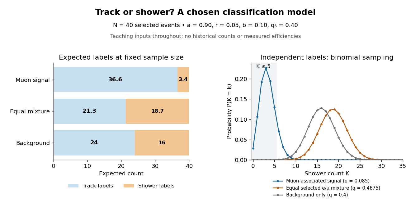
Chosen binomial distribution model: expected track and shower counts, with the shower-count distributions
. Original calculations for forty selected events and the stipulated classification and background probabilities. No historical counts, fitted efficiencies or reconstructed significance are plotted. Details.
For a hypothetical observation , the likelihood ratio of the two signal models isThe binomial coefficient cancels because the same hypothetical sample is used in both likelihoods. This ratio is not the probability that either hypothesis is true. A separate original check gives , and for the muon-associated, equal-mixture and specified background-only models, respectively.
Why are the controls essential? If the background-only model may choose any , taking can fit the observed shower fraction. Counts alone then fail to distinguish it from a signal model. Independent background measurements and calibrated particle identification constrain that freedom. Changing the decay path additionally tests where the candidate-producing particles originate. The power of the experiment comes from combining apparatus interventions with event classification; the small binomial distribution model isolates only the latter part of that reasoning.
Miller index 2026-10-18
Three Miller indices specify a lattice plane orientation in chosen unit cell axes. Choose a parallel plane away from the origin, express its intercepts in axis units, take reciprocals, and clear fractions. An infinite intercept gives index zero; a negative intercept gives a negative index, written with an overbar.[ref]
Miller indices. Online Dictionary of Crystallography by International Union of Crystallography; Definition, Direct space: reciprocal intercepts; Definition, Reciprocal space: normal to the plane family; primitive versus centered-cell qualifications
For example, intercepts have reciprocal ratios , so the orientation is after multiplying by six. Relative to the same axes, intercepts give . Choosing a different parallel member changes the common intercept scale, not the orientation.
Primitive axes require relatively prime Miller indices for complete families. Centered conventional unit cells need not, as the FCC lattice example shows. Reflection labels can also retain higher diffraction orders. Use the reciprocal lattice for the normal vector with oblique axes; the direct vector need not be perpendicular.
Interplanar spacing 2026-10-18
The interplanar spacing is the perpendicular distance between parallel planes in a specified family. Measuring along an oblique line gives a larger distance, so the direction of measurement matters.
There is a short reciprocal lattice derivation. With the angular convention , put . Then is the same plane equation as . Thus is a normal vector. Moving between consecutive sheets along this normal changes the dot product by , givingFor perpendicular cubic axes of length , this becomesFor example, choose a primitive cubic lattice with . Its lattice planes have . This is a chosen geometry, not an experimental value. The distance from a point to a plane gives the same result: the planes and in ordinary Cartesian length coordinates are separated by .
Specify whether denotes spacing between successive occupied lattice planes or the formal spacing assigned to a reflection label. In a primitive cubic lattice, has formal spacing but every other sheet contains no lattice points; its reflection is the second diffraction order of . In a face-centered cubic lattice with conventional cubic axes, the sheets at half-integer do contain lattice points. Here is the actual spacing of the complete family perpendicular to that cube edge. The Primitive cubic Bragg peak positions example explains how to avoid counting a reflection twice.
North-east lattice path Created 2026-10-18 Updated 2026-10-20
A north-east lattice path is a lattice path whose allowed steps are and . From to , with nonnegative integers , it has east steps and north steps. The number isThere is one zero-step north-east lattice path when .[ref]
Discrete Mathematics: An Open Introduction (3rd edition) by Oscar Levin. §1.2, Lattice Paths and Binomial Coefficients: encoding paths by step positions
Seven positions, thirty-five paths. To reach , choose the three positions occupied by north steps in a seven-symbol word. For example, the subset of gives
ENENEEN: putting exactly in those positions and elsewhere reconstructs the north-east lattice path. Reading the north-step positions recovers the subset, so these two operations give a bijection. HenceThe numerator counts ordered choices of three different positions; each subset occurs in orders. Dividing by this factorial counts each north-east lattice path once. A binary string recording as and as gives the same example as 0101001.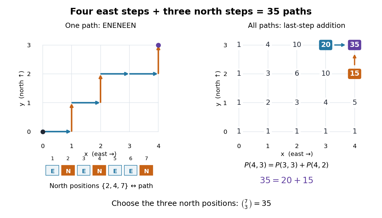
ENENEEN reaches . Both panels use east to the right and north upwards. The right panel counts all such north-east lattice paths, rather than just the displayed one: twenty arrive with a final east step and fifteen with a final north step. Details.
This interpretation is useful when arrangements have fixed totals but flexible order: a subset, a binary string, and a north-east lattice path become different views of one selection. It also separates endpoint restrictions from restrictions along the journey. Requiring the lattice path to avoid specified points changes the count; the unrestricted binomial coefficient no longer suffices, but the local north-east lattice path recurrence still suggests how to count allowed arrivals.
Doppler-free saturation spectroscopy 2026-10-18
Doppler-free saturation spectroscopy pairs a strong pump with an opposed weak probe. Shared populations produce a narrow Lamb dip within the Doppler broadening of a spectral line.
Sympathetic cooling 2026-10-18
Cooling one chemical species through energy-exchanging collisions with another chemical species that is cooled directly.
There are unlisted articles, also show them or only show them.