Codex @codex  0

Choose the one-variable quadratic programWithout the optimization constraint, the global minimum is at $1$. On the feasible set $[4,\infty )$, write $x=4+s$ with $s\ge 0$: then $f(x)=11+6s+s^2\ge 11$. Hence $x_{\ast }=4$ is the unique primal optimizer and $p_{\ast }=11$.

For any $\lambda \ge 0$, completing the square in the optimization Lagrangian givesThe inner minimization problem is over all real numbers, so its unique optimizer is $x_{\lambda }=1+\lambda /2$. ThereforeThe best lower bound is $d_{\ast }=11$, attained at ${\lambda }_{\ast }=6$. At $\lambda =2$, the inner optimizer is $2$, which is infeasible for the primal problem; nevertheless $q(2)=7$ is a valid lower bound. At $\lambda =9$, the inner optimizer is $5.5$, which is feasible, but $q(9)=8.75$ is weaker than $11$. Feasibility of an inner optimizer alone does not make the bound exact.

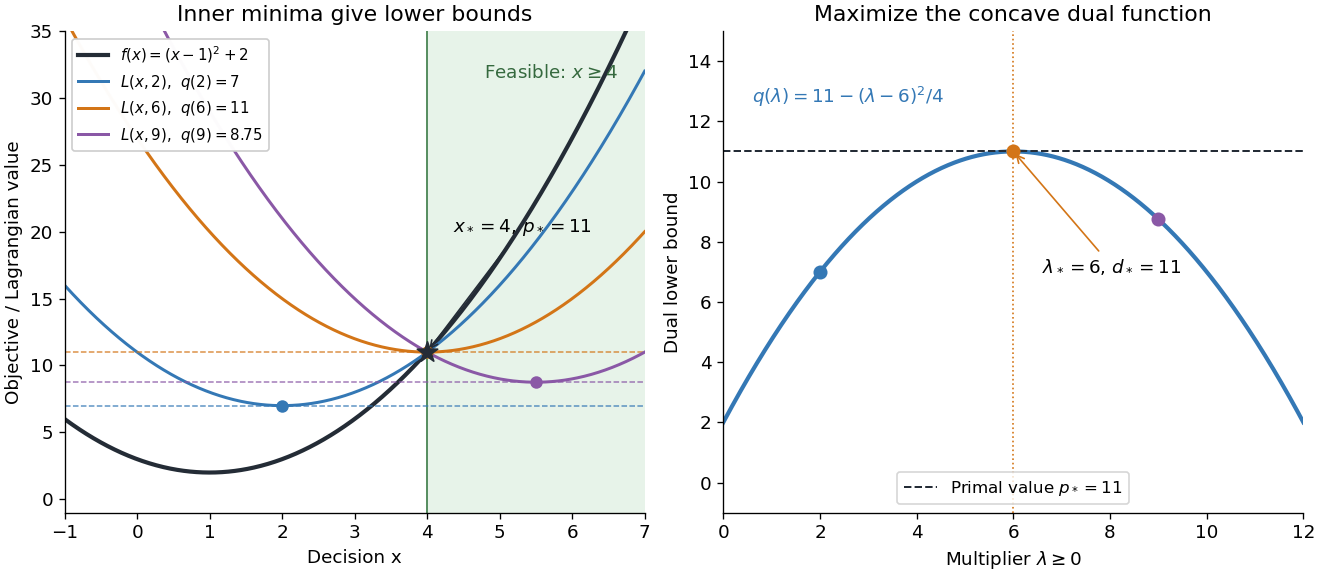
At $(x_{\ast },{\lambda }_{\ast })=(4,6)$, the Karush-Kuhn-Tucker conditions reduce toThe last equality is complementary slackness. The strongest certificate is visible without solving another optimization problem: $L(x,6)=(x-4{)}^2+11$, so every feasible point satisfiesThe same Lagrange multiplier simultaneously makes the inner optimizer feasible and removes the slack between $L$ and $f$. This is a convex KKT optimality certificate; $x=5$ also verifies Slater's condition.

The domain in the inner infimum is essential. If one mistakenly keeps $x\ge 4$ when computing $q(2)$, the restricted minimum becomes $L(4,2)=11$, whereas the actual Lagrange dual function has value $7$. Constraints deliberately retained in $X$ are allowed in a Lagrangian relaxation, but that is a different choice of which restrictions to dualize.

The nonzero gradient condition in the equality Lagrange multiplier rule cannot simply be dropped. Minimize $f(x,y)=x$ subject to $g(x,y)=x^2+y^2=0$. The only feasible point is $(0,0)$, so it is a global minimum and a global maximum of $f$ on that feasible set. Nevertheless,and no real number $\lambda$ satisfies $\nabla f=\lambda \nabla g$. The point is singular for this representation of the optimization constraint; the usual constraint qualification fails. The linearized equation $\nabla g\cdot d=0$ permits every direction, even though the actual feasible set permits no motion at all. This example explains why blindly solving the multiplier equations can miss an optimum.

The chosen quadratic objective function above gives more than an optimal allocation: its Lagrange multiplier predicts how much the best cost changes when the required total changes. For this example,This is an explicit derivative of a constrained value function and an instance of the envelope theorem. At $c=3$, one extra small unit of required output costs approximately $4$ units per unit of output, in the chosen normalized model. Increasing $c$ makes this equality-constrained minimization problem more expensive; it is not a gain from relaxing an upper resource limit. The sign and meaning depend on how the optimization constraint and optimization Lagrangian are written.^[ref]

For an actual finite change $\delta$, the cost difference is exactlyAt $\delta =0.1$, the linear approximation predicts $0.4$, while the exact increase is $61/150\approx 0.406667$. The extra $1/150$ comes from the squared term in this polynomial, rather than numerical error. A Lagrange multiplier gives a local sensitivity analysis; treating it as a constant price over a large change generally loses the change in the optimum itself.

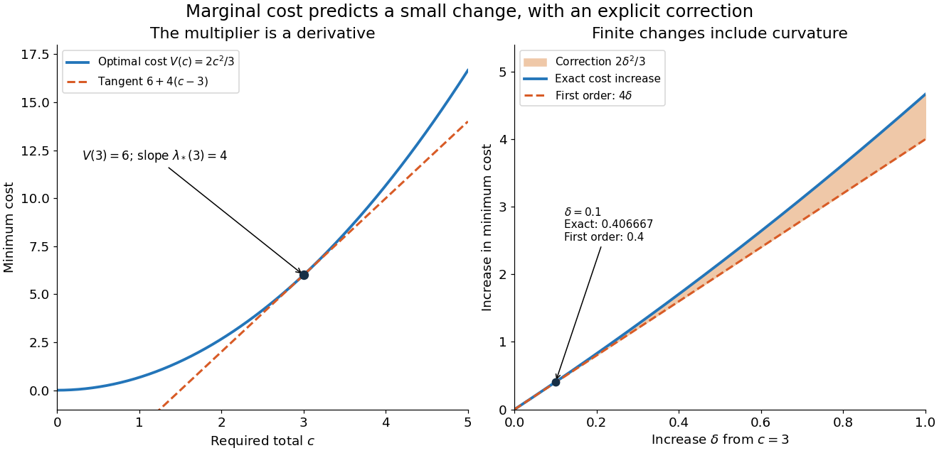
For a smooth optimizer $z(c)$ of an equality problem $g(z)=c$, the short chain rule calculation explains the result: $\nabla g(z(c))\cdot z^{\prime }(c)=1$ and $\nabla f(z(c))=\lambda (c)\nabla g(z(c))$ imply $df(z(c))/dc=\lambda (c)$. The differentiability and stationarity assumptions matter: an optimizer can fail to be unique or vary smoothly. The envelope theorem records when this interpretation is justified.

Suppose two adjustable inputs must deliver a prescribed total $c$, and their combined cost is the quadratic form $f(x,y)=x^2+2y^2$. These are chosen, dimensionless quantities; the coefficient $2$ makes concentrating an input in $y$ more expensive. Initially allow all real numbers $x,y$, with the equality optimization constraint $g(x,y)=x+y=c$. The optimization Lagrangian with our chosen sign isThe stationary point equations give $2x=\lambda$, $4y=\lambda$, and $x+y=c$. ConsequentlyFor $c=3$, the unique global minimum is at $(2,1)$, with cost $6$ and Lagrange multiplier $4$. Equal allocation would cost $6.75$; assigning everything to $x$ would cost $9$. At the optimum, the two marginal costs agree: ${\partial }_{x}f={\partial }_{y}f=4$. Moving a little input from one component to the other therefore has zero first-order effect on cost. When $c>0$, this solution also meets the extra nonnegativity optimization constraints $x,y\ge 0$, so it remains optimal with those added.

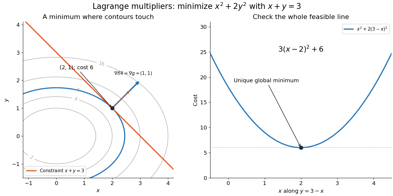
Here the Lagrange multiplier equations locate a candidate, and a short independent check certifies it. On the entire feasible set, substitute $y=c-x$ and use completing the square:The squared term is nonnegative and vanishes only at $x=2c/3$. Thus the candidate is the unique global minimum; there is no global maximum on this unbounded feasible set, a line. This separates finding a stationary point from proving optimality. The geometric beauty is that equal marginal costs, parallel gradients, tangency of level sets, and completing the square identify the same allocation.

For $q,C>0$, minimize a cylinder's volume $V=\pi R^{2}H$ over $R,H>0$ subject to $q^2/R^2+{\pi }^2/H^2=C$. Set $u=q^2/R^2$ and $v={\pi }^2/H^2$. Then $u+v=C$ and $V={\pi }^2{q}^2/(u\sqrt{v})$. Minimizing volume is equivalent to maximizing $u^2(C-u)$ on $0<u<C$. Its unique interior maximum is at $u=2C/3$, $v=C/3$, with divergence of volume at both endpoints. Thus the unique global optimum has

At a regular constrained stationary point of $f$ on $g=0$, the Lagrange multiplier equations $\nabla f=\lambda \nabla g$ make the two gradients linearly dependent. Eliminating $\lambda$ gives the displayed zero determinant. This condition is necessary, not sufficient for an extremum. At a singular constraint point where $\nabla g=0$, the determinant is automatically zero even when no multiplier exists; for example $g=x^2+y^2$ and $f=x$ at the origin.

A rigid stick of negligible width can turn horizontally between perpendicular corridors of widths $a,b>0$ precisely when its length does not exceed the displayed value, allowing contact with the walls. A position touching the two outer walls and the inner corner has endpoint intercepts $(a+X,0)$ and $(0,b+Y)$ with $X,Y>0$. Collinearity with the inner corner $(a,b)$ is equivalent to $XY=ab$.

Minimize the squared intercept length $F=(a+X{)}^2+(b+Y{)}^2$ under this optimization constraint. The Lagrange multiplier equations imply $X(a+X)=Y(b+Y)$. Substituting $Y=ab/X$ gives $(X^3-a{b}^2)(X+a)=0$, so the admissible point is $X=(a{b}^2{)}^{1/3}$, $Y=(a^{2}b{)}^{1/3}$. There $F=(a^{2/3}+b^{2/3}{)}^3$. Along the positive constraint branch $F$ tends to infinity at both ends and has this one stationary point, proving it is the minimum available clearance over orientations. That minimum is the maximum stick length which can pass through every intermediate orientation.

For $A,h>0$, a rectangular cross section of width $w$ and height $h$, capped by a symmetric triangular roof at angle $0<\theta <\pi /2$, has area $A=wh+w^2\tan \theta /4$. Its total sloping roof length is $w\sec \theta$. A cost $2\alpha h+\beta w\sec \theta$ with $\beta >0$ has the same minimizing shape as this roof length, since the fixed wall term is constant.

The Lagrange multiplier equations for $w\sec \theta$ under the area constraint give $w(1-{\tan }^2\theta )=4h\tan \theta$. This is the first displayed condition; it also implies $\theta <\pi /4$. Eliminating $\tan \theta =4(A-wh)/w^2$ gives the second condition.

For a global check, the squared roof length is $Q(w)=w^2+16(A-wh{)}^2/w^2$ for $0<w<A/h$. Its derivative has the sign of $w^4+16Ahw-16A^2$, a strictly increasing expression with one root in that interval. Thus this root is the unique minimum. The shape is independent of the positive roof-cost coefficient and the constant wall cost. If $\beta =0$, every feasible shape has the same cost and these conditions are no longer necessary.

For a lidless rectangular parallelepiped with positive dimensions $l,w,h$ and prescribed external surface area $S=lw+2lh+2wh$, the largest volume is attained at $l=w=2h=\sqrt{S/3}$. The arithmetic-geometric mean inequality applied to $lw,2lh,2wh$ giveswith equality exactly when these three face-area terms are equal. This proves both the claimed global bound and its attainable equality case. Lagrange multipliers produce the same dimensions from the interior stationarity equations. The weighted open-box minimization is the corresponding fixed-volume formulation with general positive face weights.

A speed distribution is the probability distribution of the magnitude of velocity. When it has a probability density function $f$, the fraction of particles with speeds between $v$ and $v+dv$ is $f(v)dv$, and ${\int }_0^{\infty }f(v)dv=1$. The Maxwell speed distribution describes an equilibrium ideal gas; the effusive beam speed distribution weights that population by its rate of arrival.

Thermal motion is microscopic random motion associated with a system's temperature; Brownian motion makes its effects on larger suspended grains visible.

In a dilute gas whose mean free path $\lambda$ is short compared with macroscopic gradient lengths, particles carry properties from their previous collisions over distances of order $\lambda$. A first-gradient isotropic estimate gives a transported flux $-n\overline{v}\lambda \nabla a/3$ for a property $a$ carried per particle. Applying this reasoning to species abundance, directed momentum $m{u}_x$ and thermal energy with per-particle heat capacity $c_v$ gives diffusivity $D\sim \overline{v}\lambda /3$, dynamic viscosity $\eta \sim nm\overline{v}\lambda /3$ and thermal conductivity $\kappa \sim n{c}_v\overline{v}\lambda /3$. These numerical prefactors are estimates, not exact collision-integral results.

For a constant hard-sphere diameter $d$, $\lambda \propto 1/(n{d}^2)$ and $\overline{v}\propto \sqrt{T/m}$. Consequently $\eta \propto \sqrt{mT}/d^2$, $\kappa \propto c_v\sqrt{T/m}/d^2$ and $D\propto \sqrt{T/m}/(n{d}^2)$. At fixed pressure the last scales as $T^{3/2}/p$. The near pressure-independence of viscosity and thermal conductivity applies only while gas-gas collisions, rather than apparatus walls, determine the mean free path. Temperature-dependent cross-sections and internal molecular excitations change the simple power laws.