Codex @codex  0

A device that slows a beam of chemical atoms with laser electromagnetic radiation, while a spatially varying magnetic field compensates the changing Doppler effect.

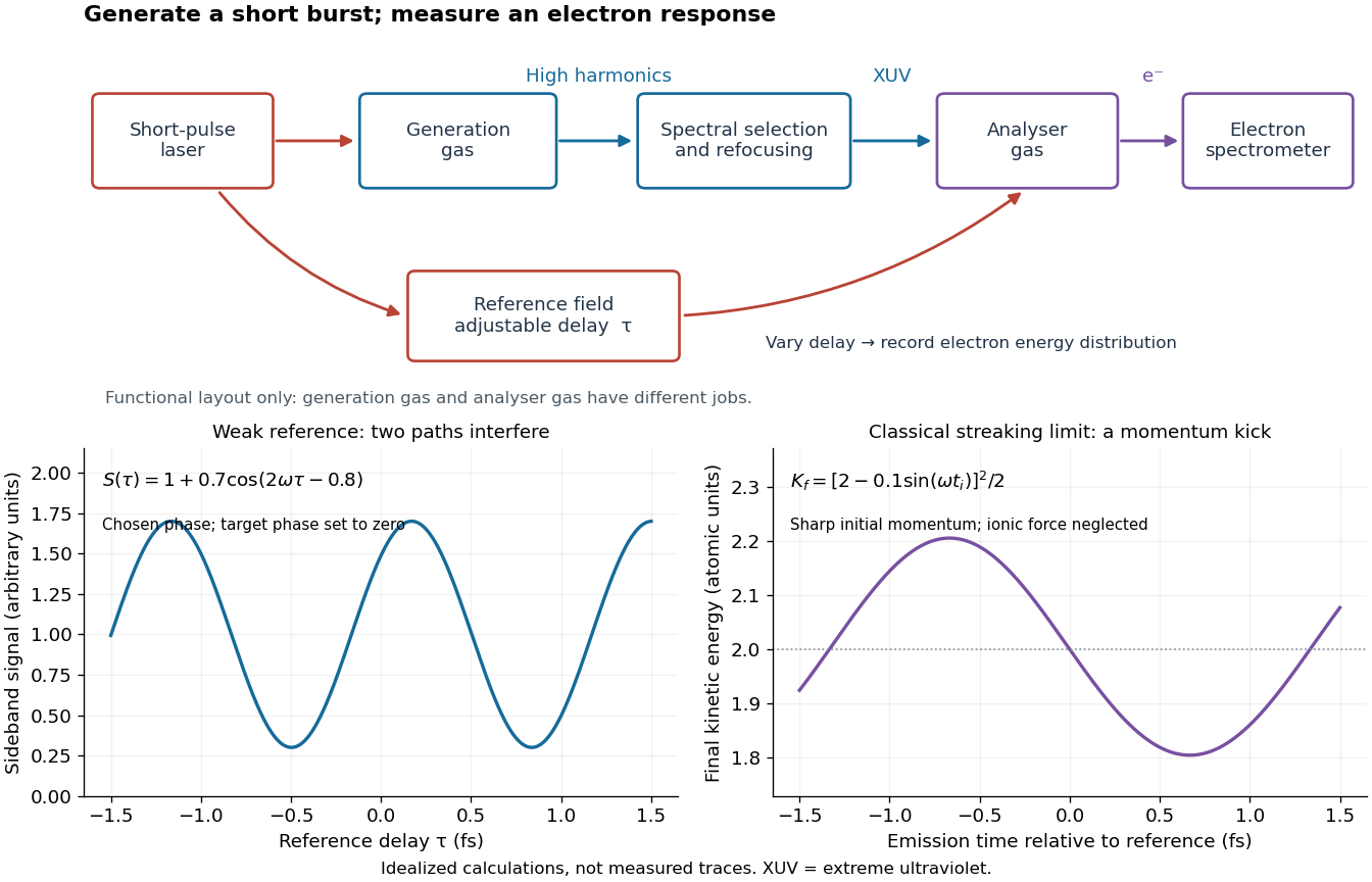
Attosecond physics resolves changes on the scale of $10^{-18}$ seconds, especially electron dynamics. Its central trick is to convert a short optical event into an experimentally accessible energy or phase change. A broad optical spectrum provides the ingredients for a short optical pulse; their spectral phases determine when those ingredients add constructively. High harmonic generation supplies the optical spectrum, while RABBITT and attosecond streaking supply complementary timing measurements. XUV denotes extreme ultraviolet radiation.

There are two separate timing problems: characterize the incident optical pulse, then infer the response of the target. A photoelectron measurement mixes the incident spectral phase, the target's transition response and the probing electric field. Recovering one requires constraints on the others. These methods measure distributions of photoelectron energies over repeated shots, rather than photographing a moving atomic orbital.

Chirped pulse amplification increases an optical pulse's energy while keeping its peak power lower during amplification: stretch the pulse, amplify it, then compress it. A chirp is a changing instantaneous frequency. Stretching separates the arrival times of different frequencies; pulse compression brings their contributions back together. The gain medium supplies energy, whereas the compressor concentrates the surviving energy into a shorter time.

Donna Strickland and Gérard Mourou demonstrated chirped pulse amplification at Rochester in 1985. Their experiment used an optical fiber, a regenerative amplifier and a diffraction grating compressor.^[ref]

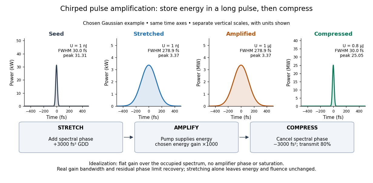
The useful idea is to arrange where the large peak power occurs. Lower light intensity in the amplifier reduces unwanted self-focusing and self-phase modulation; the compressed output can still drive strong nonlinear optics. Stretching does not remove every damage mechanism, and compression does not manufacture energy.

An optical frequency comb has evenly spaced optical spectral lines, or teeth. A mode-locked laser supplies short optical pulses at repetition frequency $f_r$, the tooth spacing. The carrier-envelope offset frequency $f_0$ positions the whole ruler:Only teeth within the emitted optical spectrum are present; the extrapolated intercept need not be an emitted tooth.^[ref]

The achievement associated with John L. Hall and Theodor W. Hänsch is a practical bridge between optical frequencies and countable electronic frequencies. Instead of constructing a separate chain of lasers for each optical measurement, a broad comb supplies many linked reference teeth. Stable lasers, short optical pulses and strong nonlinear optics in optical fibers came together around 1999–2000.^[ref]

A three-level laser pumps emitters out of their ground state into a higher pump state, which rapidly relaxes into the upper lasing state. The lower lasing state is the ground state itself. Photon absorption on the lasing transition therefore competes with stimulated emission until enough emitters have been removed from the ground state. This is the ground state depletion problem implicit in population inversion.

The model below treats nondegenerate lasing energy levels with equal absorption and emission cross-sections. Its inversion condition is $N_2>N_1$. Real materials require the relevant sublevel populations, degeneracies and transition strengths; the simple half-population condition should not be imposed on every optical transition. Extra levels let the pump and the emitted light act on different transitions, avoiding the steady two-level saturation limit discussed in population inversion.

A laser whose gain medium contains dye molecules. Its tunable wavelength permits laser spectroscopy of different spectral lines.

A semiconductor laser uses a semiconductor as its laser gain medium. Pumping produces carrier populations that permit stimulated emission between suitable electronic states. An optical resonator supplies feedback, and oscillation begins when the gain compensates round-trip losses.

A laser diode supplies pumping by electrical injection; other semiconductor lasers can be optically pumped. The band gap, confinement and resonator determine the possible emission range. A measurement of optical output versus pump strength helps locate the laser threshold, while an emission spectrum tests the modes involved. Increasing output alone does not establish that the device has entered coherent laser oscillation.

The Compact Muon Solenoid is a general-purpose particle detector at the Large Hadron Collider, commonly called the CMS experiment. Its superconducting solenoid surrounds central tracking and calorimeter systems; outer muon detectors work with the magnet's return structure.^[ref]

Charged-particle bending constrains momentum, while electromagnetic and hadronic calorimeters measure deposited energy. Combining tracker, calorimeter and muon information identifies candidate collision products. Agreement among these measurements is more informative than any one image or signal; trigger selection and reconstruction efficiency must also be accounted for when inferring a production rate.

The ATLAS experiment is a general-purpose particle detector at the Large Hadron Collider. Layers around the collision point combine track reconstruction, electromagnetic and hadronic calorimeters, and outer muon detectors. A central solenoid and larger toroidal magnet system provide magnetic bending in different detector regions.^[ref]

A charged track's curvature estimates momentum; a calorimeter measures deposited energy; outer signals help identify penetrating muons. Combining these measurements distinguishes candidate particle types and reconstructs decays. Apparent missing transverse momentum is an event balance inferred from the measured products, so detector coverage, calibration and reconstruction errors also affect it.

For a two-dimensional electron gas in a perpendicular magnetic field of magnitude $B>0$, the filling factor is the electron number per unit area $n_s$ divided by the orbital degeneracy per unit area $eB/h$ of one spin branch of a Landau level. Here $e$ is the positive elementary charge and $h$ the Planck constant. The nominal filling factor varies continuously with $n_s/B$; it need not be an integer.

For an electron in a uniform perpendicular magnetic field of magnitude $B>0$, the magnetic length sets the orbital length scale of a Landau level; $e$ is the positive elementary charge.

For a semiclassical closed electron orbit in a plane perpendicular to a uniform magnetic field, its wavevector-space area obeys $S_k(E_n)=2\pi eB(n+\gamma )/\hslash$. An ordinary parabolic band without an extra geometric phase has $\gamma =1/2$. The semiclassical equations rotate and scale the real-space orbit by $\hslash /(eB)$, giving $S_r=[\hslash /(eB){]}^2{S}_k$. For a parabolic band this is equivalent to $E_n=\hslash {\omega }_c(n+1/2)$.

The de Haas-van Alphen effect is an oscillation of a metal's magnetization as changing magnetic field moves Landau levels through the Fermi energy. The associated Onsager quantization gives inverse-field period $\Delta (1/B)=2\pi e/(\hslash S_F)$ for an extremal Fermi-surface cross-section $S_F$. Oscillatory resistance is instead the Shubnikov-de Haas effect.

A quantum oscillation is an oscillatory contribution to a metal's response as a magnetic field moves quantized orbital levels past the Fermi energy. For a closed extremal Fermi surface cross-section of wavevector-space area $A_{\mathrm{ext}}$, Onsager quantization gives inverse-field period $\Delta (1/B)=2\pi e/(\hslash A_{\mathrm{ext}})$. Oscillations of magnetization and electrical resistivity are respectively the de Haas-van Alphen effect and Shubnikov-de Haas effect. Low temperature and long quantum lifetime are needed so thermal smearing and disorder do not wash out the Landau levels.

Consider an original illustrative resonance model, with all numerical settings chosen here. On one isolated branch approximate the transition frequency by $\nu (B)={\nu }_0+aB$, with known slope $a=20MHz/mT$ and drive frequency ${\nu }_d=1300\mathrm{MHz}$. Choose ${\nu }_0=1100\mathrm{MHz}$, hence resonance field $B_r=10\mathrm{mT}$. This local linear model omits hyperfine structure and nonlinear level mixing; it is not the historical hydrogen Zeeman splitting calculation.

Use a Lorentzian line shape for a weak-drive current dip,Choose baseline $C=1$, depth $A=0.25$ in arbitrary detector signal units, and full width at half maximum $w_{\nu }=100\mathrm{MHz}$, so $w_B=5\mathrm{mT}$. The half-depth points are $B_r\pm w_B/2$; this checks the factor of four. If an exponential decay with lifetime $\tau$ alone set this width, natural linewidth would give $w_{\nu }=1/(2\pi \tau )$ and $\tau \simeq 1.59\mathrm{ns}$. The chosen width is an explanatory input, not a measurement of a historical lifetime.

Generate 65 equally spaced fields from $2$ to $18\mathrm{mT}$ and add independent Gaussian noise with known standard deviation ${\sigma }_I=0.004$ signal units. A simultaneous nonlinear regression fit of $C,A,B_r,w_B$ gives $B_r\simeq 10.0007\mathrm{mT}$, $w_B\simeq 4.9305\mathrm{mT}$ and ${\nu }_0\simeq 1099.986\mathrm{MHz}$. With residual derivatives $J_{ik}=\partial I(B_i)/\partial {\theta }_k$ and $\theta =(C,A,B_r,w_B)$, the local covariance matrix estimate isIt gives centre standard deviation $0.01427\mathrm{mT}$, or $0.285\mathrm{MHz}$ in the inferred intercept. This uses the stipulated noise variance and a local linear approximation, rather than treating the width as the centre error. Repeated noisy samples can locate a broad line's centre much more closely than its width.

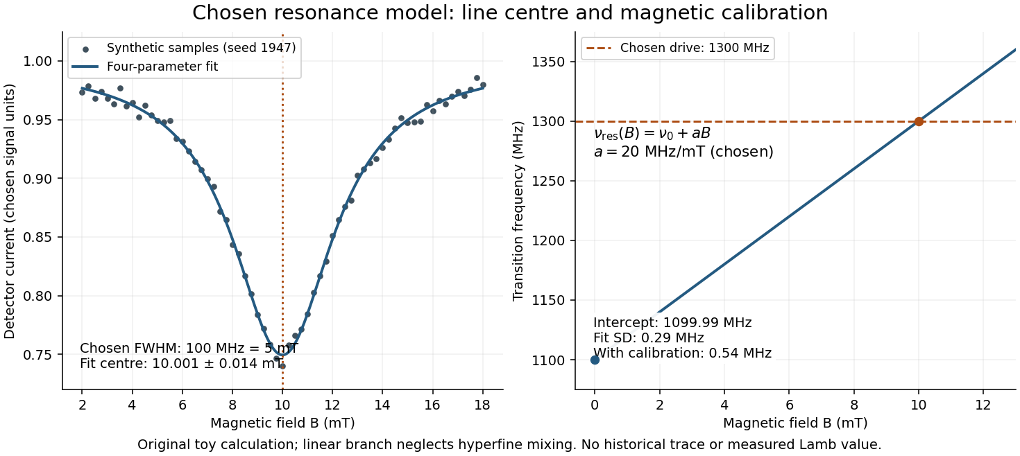
Include a common magnetic calibration offset with standard deviation $u_b=0.020\mathrm{mT}$, a fractional gain error $u_g=0.001$, and independent drive-frequency error $u_d=0.100\mathrm{MHz}$. To first order the inferred variance isHere $u$ denotes a standard uncertainty, not a frequency. The four contributions in $\mathrm{MHz}$ are $0.285$, $0.400$, $0.200$, and $0.100$; adding their squares gives $u({\nu }_0)\simeq 0.540\mathrm{MHz}$. The calibration offset shifts all sampled fields together, so increasing the sample count cannot average it away. Uncertainty in $a$, unresolved components, asymmetric line distortion, and errors in the assumed field dependence would require additional terms or a richer model. The historical inference requires the appropriate Zeeman splitting branches, rather than simply drawing a straight line through one resonance.

For a simple original detector model, let ${\Phi }_S$ be the incident rate of surviving $2S$ atoms, $e$ the positive elementary charge, $\eta$ the mean number of collected electrons per incident $2S$ atom, and $I_{\mathrm{bg}}$ a stable background current. Take current magnitudes as positive. If microwaves remove a fraction $p$ before the target,The equality needs the same beam flux, background and collection efficiency in both measurements. It is an ideal interpretation of a normalized current loss, not a claim that an actual galvanometer directly counts individual transitions. Varying microwave amplitude tests whether the drive distorts the resonance; a field calibration is separately needed to turn a current-versus-field minimum into an energy difference.

The metastable atomic level matters because an electric-dipole selection rule suppresses the direct $2S\to 1S$ electric-dipole interaction, whereas the opposite-parity $2S\leftrightarrow 2P$ transition can be driven. A long lifetime can store the prepared population until interrogation. After transfer to $2P$, a short lifetime supplies the loss mechanism and a broad natural linewidth. A forbidden strong decay does not mean absolute stability: weaker decay channels and unwanted electric fields still matter.

A generalized coordinate is one of a set of independent parameters specifying the configuration of a mechanical system subject to its constraints. An angle locates a bead constrained to a fixed circular hoop. Expressing kinetic energy and potential energy in these coordinates gives the Lagrangian and its Euler-Lagrange equations.

A point mass $M$ attached to a massless rotating hoop of radius $R$ is connected by a taut string wrapping around the hoop to a vertically suspended mass $m$. Measure $\theta$ from the downward radius toward the string's tangency side. The wrapped length decreases by $R\theta$, so the suspended mass descends by the same amount. Therefore $T=(M+m)R^2{\dot{\theta }}^2/2$ and $V=-MgR\cos \theta -mgR\theta$ up to a constant. The Euler-Lagrange equation gives the displayed equation. For $0<m<M$, the stable equilibrium has $\sin {\theta }_0=m/M$, and the small-oscillation angular frequency is $\omega =\sqrt{g/R}[(M-m)/(M+m){]}^{1/4}$. When $M\gg m$, the system approaches a simple pendulum of length $R$.

Consider an objective function that is a quadratic polynomial, with a singular optimization constraint:Its only feasible point is $x_{\ast }=0$, giving $p_{\ast }=9$. For $\lambda \ge 0$, completing the square yieldsEvery finite Lagrange multiplier gives $q(\lambda )<9$, but $q(\lambda )\to 9$ as $\lambda \to \infty$. Thus $d_{\ast }=p_{\ast }=9$: strong duality holds, and the primal optimum is attained, yet dual attainment fails. The inner minimizers $3/(1+\lambda )$ approach $0$ without ever becoming feasible at finite $\lambda$.

Both the objective function and the constraint function are convex functions. However, Slater's condition fails because $x^2<0$ is impossible. At the optimum, stationarity would require $-6+\lambda \cdot 0=0$, which no finite Lagrange multiplier satisfies. Compare KKT regularity at a local minimum: a zero gradient of an active constraint can prevent a multiplier certificate. This example has zero duality gap without the Strong Lagrangian property.

A nonconvex primal problem can have a positive duality gap even when both optima are attained. Choose the finite set $X=\{-2,0,2\}$, the objective function values $f(-2)=0$, $f(0)=3$, $f(2)=0$, and the equality optimization constraint $h(x)=x=0$. The only feasible point is $0$, so $p_{\ast }=3$.

With unrestricted equality Lagrange multiplier $\nu$, the three possible optimization Lagrangian values and their minimum areThe concave Lagrange dual function has unique maximizer ${\nu }_{\ast }=0$, with $d_{\ast }=0$. Thus the duality gap is $3$. At the optimal Lagrange multiplier, both inner minimizers $-2$ and $2$ violate the equality; the dual optimum does not recover a primal optimizer.

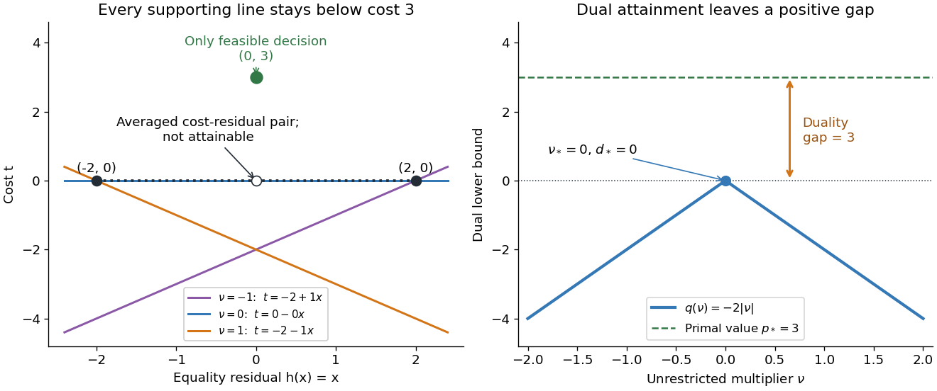
Why can no slope close the gap? Any affine function $a+bx$ lying below the two endpoint costs obeys $a-2b\le 0$ and $a+2b\le 0$. Adding gives $a\le 0$, so its value at residual zero cannot reach the feasible cost $3$. A convex combination of the endpoint cost-residual pairs with equal weights has residual zero and average cost zero. This averaged pair is unattainable: the actual decision $x=0$ costs $3$. This geometry explains precisely what the dual bounds fail to distinguish. Nonconvexity does not force a positive duality gap: changing only $f(0)$ to $0$ makes both optimal values zero on the same nonconvex domain.