
For a block sliding right on a stationary horizontal plane, take rightward acceleration as positive. A gauge reading for a pull at angle above horizontal has horizontal component and upward component . With no vertical acceleration or other forces, Newton's second law givesand thereforeThis inference requires continued contact with and rightward contact slip, so its numerator must be nonnegative. An upward pull reduces normal force; a downward pull, represented by , increases it. The horizontal constant-velocity formula is the special case , .
For the original , model, an upward pull at maintaining constant velocity needsDividing this gauge reading by would give about , rather than : the gauge reads the full inclined force, and the pull has changed the normal force.
Even with a horizontal pull, an accelerating measurement needs the correction: . In the same model, a horizontal pull produces while the block slides right; subtracting recovers the kinetic friction. Dividing the uncorrected reading by instead gives about . Measure acceleration in an inertial frame, along the sliding direction, over the same interval as the gauge reading. These corrections follow from the force balance, independently of whether the resulting coefficient of kinetic friction is constant across runs.
// Target: classical-mechanics.bigb
Load dependence of kinetic friction 2026-10-14
Changing the added mass while retaining the same contact pair and sliding speed tests whether a constant coefficient of kinetic friction is a useful model. Compute for each level horizontal run, and plot the mean sliding force vertically against normal force horizontally. The constant-coefficient prediction is a straight line through the origin; its slope is . This extracts a ratio from several loads rather than relying on one reading.
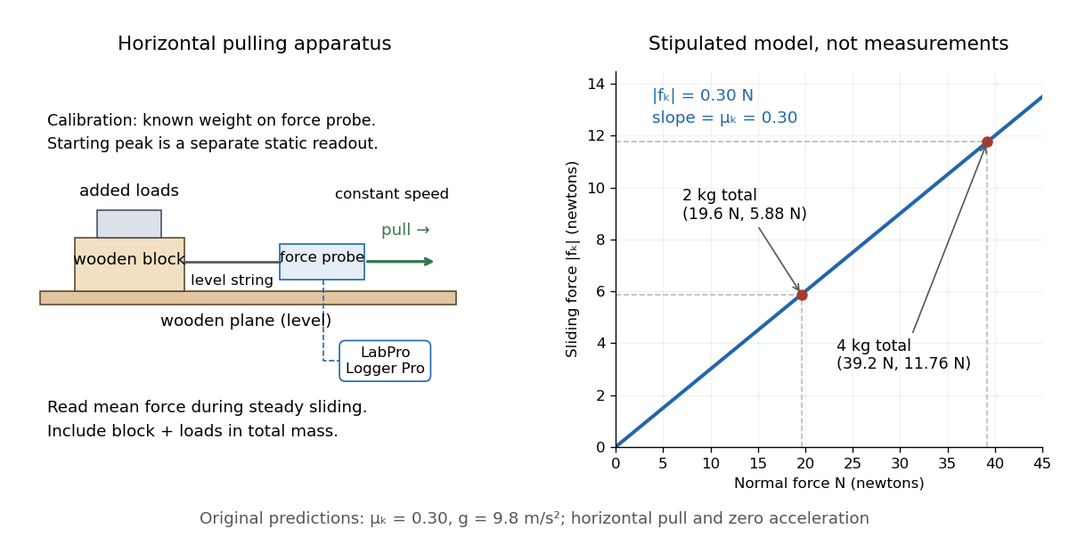
Horizontal wooden-block force-probe apparatus and original load model: 19.6 N and 39.2 N normal loads predict 5.88 N and 11.76 N sliding forces
. Details. 
The apparatus sketch identifies the contact pair and horizontal pull used by the cited laboratory procedure. The plotted line and points are the original stipulated model from coefficient of kinetic friction, not laboratory data. The two model points giveIn actual measurements, a linear regression can expose an unexplained intercept . A nonzero intercept calls for checking the gauge zero, other resisting forces and the contact model; forcing the line through zero can hide those problems. Conversely, constant ratios within measurement error support the approximation only over the loads, speeds and surface conditions tested. A load sweep alone cannot establish independence from contact area or sliding speed; those require separate controlled variations.
A force gauge reads the pulling force. For horizontal straight-line sliding at constant velocity, its reading equals the opposing kinetic friction magnitude, provided these are the only horizontal forces. For total supported mass , including added loads, , so a mean sliding reading gives . The important readout is the sustained sliding force after the starting peak; the peak belongs to the static friction threshold.
The University of Mississippi's Experiment 6 uses a wooden block on a wooden plane, a triple-beam balance, added masses, and a dual-range 50 N force probe connected through LabPro to Logger Pro. Its procedure calibrates the probe with a load on a hanger, entering the corresponding force in newtons, and measures the block's mass separately. With the plane horizontal, it starts with on the block and pulls horizontally at constant speed. The recorded force trace has a starting peak; the procedure selects the subsequent constant-force interval and takes its mean. It repeats with increments up to added, then plots sliding force against normal force to estimate the coefficient of kinetic friction from the slope.[ref]
Experiment 6: The Coefficient of Friction (University of Mississippi teaching laboratory). Experiment 6, The Coefficient of Friction, PDF pp. 1–2: Equipment, Objectives, Procedure steps 1–7
For a replication, check the gauge's zero with the string slack and its response to known gravitational weights; zeroing alone does not check its scale. Keep the plane level, the pull parallel to it, and the block face and track region consistent. Specify the contacting materials and whether the surfaces are dry, cleaned or lubricated; repeat runs to see whether debris or wear changes the sliding force. Verify constant velocity independently from position versus time, rather than assuming that a flat force trace proves zero acceleration. These are proposed measurement controls, not additional observations from the laboratory writeup. Record the selected interval, variation between runs and gauge resolution as sources of measurement error.
Stop codon Created 2026-10-14 Updated 2026-10-20
In the standard genetic code, UAA, UAG and UGA are stop codons: they signal termination of biological translation rather than an amino acid assignment. See Clark, Douglas and Choi: stop codons.
A stop codon supplies no additional amino acid residue. In the constructed AUG GCU UUC UGA example, replacing UGA by UAA preserves termination after the same three amino acid residues. Replacing UUC by UAA instead terminates after methionine and alanine. These are consequences of the stated genetic code, not measurements of expression efficiency.
At a standard stop codon, a release factor promotes release of the polypeptide from the ribosome. Ordinary delivery of an amino acid by transfer RNA does not supply a “stop amino acid”.[ref]
Biology 2e by Mary Ann Clark and others. §15.5, Translation, Elongation, and Termination, paragraph beginning “Termination of translation”: stop codons and release factors
Rank-sum form of Cochran's theorem 2026-10-14
Let be real symmetric matrices with sum . Their matrix ranks sum to at least , because their ranges span . If the ranks sum to , those ranges form a direct sum. For in the range of , the identity and uniqueness of its range decomposition imply . Thus and for : the matrices are mutually orthogonal orthogonal projections. In a combined orthonormal basis, the forms for use disjoint sets of independent standard normal coordinates. They are independent chi-squared distributions with degrees of freedom equal to the ranks. Conversely, if all these forms have those chi-squared laws, their expectations and their sum give .
Universal simple-shear normal-stress identity Created 2026-10-14 Updated 2026-11-05
For simple shear, . The off-diagonal entry of is . Coaxiality of isotropic elastic stress therefore proves the identity for . At , material isotropy makes the stress isotropic, proving the same identity.
Equivariance of isotropic principal stresses Created 2026-10-14 Updated 2026-11-05
For an objective material isotropy law, permutation of the principal stretches permutes the labelled principal stresses. This follows by conjugating the left stretch tensor with signed permutation rotation matrices. Each principal stress is symmetric in the other two stretches, but need not be symmetric in all three. The law provides the example . In an invariant representation , the scalar coefficients are symmetric functions of the unordered stretches.
Unit index of a CM-field Created 2026-10-14 Updated 2026-11-05
For a CM-field, put for conjugation and . The map takes values in the cyclic group of roots of unity: all conjugates have absolute value one, and the Kronecker theorem on algebraic integers in the unit disk applies. Its kernel is , while its image on is . It therefore embeds into , a group of order two. This proves the index bound without assuming that every unit is a real unit times a root of unity.
Clutching function 2026-10-14
A clutching function is the equatorial transition map used in the clutching construction. For an oriented real vector bundle one may choose a fiber metric and orthonormal trivializations, so its clutching function takes values in the special orthogonal group.
Agglomerative hierarchical clustering 2026-10-14
Start with singleton clusters and repeatedly merge the two clusters with the smallest chosen intercluster dissimilarity. Single-linkage clustering uses the smallest cross-pair distance; complete-linkage clustering uses the largest. Merge heights and sensitivity to ties help assess a proposed number of groups.
Simple matching coefficient 2026-10-14
For binary vectors, this similarity counts agreements on both presences and absences. Its complement is the normalized Hamming distance. Whether joint absences should count as similarity depends on the application; rare-presence data may call for a different coefficient.
Dissimilarity matrix 2026-10-14
A dissimilarity matrix records pairwise separation of observations or profiles. Usually it is symmetric, nonnegative and zero on the diagonal. A metric space additionally requires the triangle inequality and separation of distinct profiles. Agglomerative hierarchical clustering can be applied to many dissimilarity matrices that are not Euclidean distance matrices; the claimed geometry must be checked separately.
Jaccard index 2026-10-14
The index measures similarity of finite sets by shared presence relative to total presence. For binary profiles it ignores joint absences, unlike the simple matching coefficient. When both sets are empty, define the similarity to be one. The complementary Jaccard distance measures dissimilarity.
K-means clustering 2026-10-14
For a prescribed number of groups, minimize within-cluster squared Euclidean distances. At fixed assignments, differentiating the objective gives the mean as the optimal centroid. At fixed centroids, assigning each point to a nearest centroid minimizes its contribution. Alternating these steps cannot increase the objective but can converge to a local optimum, so multiple starts are useful. Empty clusters and ties need an explicit handling rule. The method favors roughly spherical groups and depends on variable scaling.
Cluster in cluster analysis 2026-10-14
A cluster in cluster analysis is a nonempty group of observations treated as similar under the chosen representation and dissimilarity. A partition assigns each observation to exactly one cluster; agglomerative hierarchical clustering supplies a nested sequence of such partitions. An algorithmic cluster need not correspond to a distinct probabilistic population.
For a stable -point closed-string scattering amplitude on a genus- surface, let count complex unmarked worldsheet moduli and count complex dimensions of the worldsheet conformal Killing group. Integrating the vertex positions and moduli, then fixing positions, leaves complex integrations. The punctured Riemann surface moduli dimension identifies this as . Faddeev-Popov ghost fields and antighost insertions implement the removed zero modes and the surviving modulus measure; they do not add independently integrated worldsheet coordinates.
Compact interval 2026-10-14
A compact interval in the real numbers is either the empty set or a closed bounded interval with . Its compactness follows from the Heine-Borel theorem.
For an irreducible closed migration process with finite population , positive departure rates and routing matrix , choose positive traffic weights satisfying . On , its stationary distribution has the displayed form. For a predecessor , its weighted transition into is . Summing over gives by the traffic equation, and summing over proves global balance for a continuous-time Markov chain. The distribution need not satisfy detailed balance.
// Target: probability-and-statistics.bigb
Represent telephone lines by a closed migration process with free-line, operator and automated-service colonies. Accepted arrivals have rate when a free line exists, operators complete at rate , and automated calls complete at rate . Define andThe product-form stationary distribution of a closed migration process and Poisson arrivals see time averages give the displayed blocking probability. This extends a single-operator model without treating the independent operators as a server with rate when fewer than calls are present.
// Target: probability-and-statistics.bigb
Primitive closed geodesic 2026-10-14
A primitive closed geodesic is a closed geodesic with its smallest positive period, rather than a repeated traversal of a shorter periodic geodesic. A degree- lift of a primitive base geodesic is still primitive upstairs when its monodromy permutation has a cycle of exact length : no smaller number of traversals returns to the starting sheet.
There are unlisted articles, also show them or only show them.