
Tube the projective lines in the two summands of through the connecting neck. Their connected sum is an embedded two-sphere in the class , with self-intersection two. Its oriented normal disk bundle has Euler number two, so its boundary is the unit tangent bundle of , namely . The boundary separates the interior of the tubular neighborhood from its nonempty exterior.
// Destination: geometry-and-topology.bigb
For a connected sum of identical oriented manifolds of dimension at least three, one can permute the attachment balls in a punctured sphere and match the attached copies by their chosen parametrizations. This gives orientation-preserving diffeomorphisms realizing the permutations on the middle cohomology summands. For sums of complex projective planes, these permutations preserve the diagonal positive intersection form.
// Destination: geometry-and-topology.bigb
Connected-sum gluing of functions 2026-10-14
Remove small disks around a nondegenerate maximum of a smooth function on one closed surface and a nondegenerate minimum on another. Rescale their values so the boundary values agree with the two ends of a neck. Their regular level collars allow a strictly monotone function on the neck, with nonzero derivative, matching smoothly to both sides. The resulting connected sum has all the old critical points except the deleted maximum and minimum. This permits one degenerate torus saddle to be retained while adding ordinary handles for higher genus.
Component (graph theory) 2026-10-14
Strengthened Sylow congruence from intersections Created 2026-10-14 Updated 2026-11-05
For a finite group and a Sylow subgroup , conjugation by on all Sylow subgroups has stabilizer at : the normal Sylow subgroup of contains every -subgroup of that normalizer. Thus the orbit length is . If every has this index at least , each such orbit length is divisible by , whereas is a singleton orbit. Summing orbit lengths proves the displayed stronger integer congruence.
Normal-gamma distribution 2026-10-14
A normal-gamma conjugate prior for the mean and precision parameter of a Gaussian distribution specifies a Gamma distribution in the shape-rate convention and a conditional Gaussian distribution . Its joint probability density function is proportional to , with . For independent observations with Gaussian distribution , multiplication by the likelihood and completing the square givesand . The identity behind conjugacy is .
Infinite conjugacy class group 2026-10-14
A discrete group is ICC when every nonidentity element has an infinite conjugacy class. The trivial group satisfies this condition vacuously. It characterizes when the group von Neumann algebra is a Von Neumann factor.
Conjugacy classes of the symmetric group on three letters Created 2026-10-14 Updated 2026-10-25
The symmetric group has exactly six permutations, written using permutation cycles:Here is the identity element; , and are transpositions; and and are permutation cycles of length three. With and , rightmost-first function composition gives and . The conjugacy classes and representative centralizers are
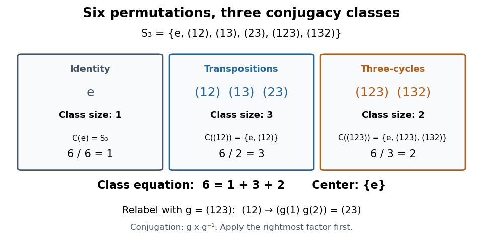
All six permutations of the symmetric group , their conjugacy classes, and representative centralizers
. Details. 
An explicit check of the conjugation with sends , , and , where each chain applies , then , then . Thus is fixed and are exchanged: . Relabelling also produces , so the three transpositions share one conjugacy class. A transposition reverses the length-three permutation cycle, since , putting both length-three permutation cycles in one conjugacy class.
Checking each of the six possible permutations against gives the displayed centralizers. Only has a one-element conjugacy class, so the center of a group here is . The class equation is . The second diagram in centralizer and normalizer uses the same and to show how preserving a cyclic subgroup differs from fixing its group generator.
Conic discriminant 2026-10-14
In characteristic different from two, a local equation for a conic bundle is with symmetric. A fibre is singular exactly when the determinant vanishes. Changing the fibre coordinates multiplies that determinant by a nonzero square, so its zero locus is intrinsically defined even when the quadratic coefficients belong to twisting line bundles.
User-network decomposition of concave utility maximization Created 2026-10-14 Updated 2026-10-31
Maximize a sum of increasing strictly concave utilities subject to , . Suppose capacities are positive, every route is nonempty, and . At its unique positive optimizer , the Karush-Kuhn-Tucker conditions give nonnegative resource congestion prices and route congestion prices . Choosing makes each user maximize at . It also makes maximize the entropy maximization for loss-network occupancy objective, since its gradient is . Thus user and network optima implement the same system optimum.
A useful motivating experiment moves a bead emitting fluorescence through the selected optical focus and records the detector signal against position. Measurement of point-spread function (PSF) for confocal fluorescence microscopy by InCheon Song and others (2005, §2 and Fig. 1) describes a laser delivered through a single-mode optical fiber, collimation, beam-size adjustment and a dichroic beam splitter. A , numerical aperture oil-immersion objective optical lens excites slide-mounted fluorescent beads and collects their emission. Emission passes a filter and collecting optical lens, then a pinhole, before an avalanche photodiode. A three-dimensional positioning stage moves the specimen. The apparatus also contains a phase plate for deliberately modified responses.[ref]
Measurement of point-spread function (PSF) for confocal fluorescence microscopy by InCheon Song and others. §2 and Fig. 1, pp. 2–3: apparatus and readout
The published comparison uses nominal bead diameters : larger beads give broader measured spots. This is a control on the finite emitter, because the image is the convolution of bead emission with the confocal point spread function. The smallest bead has weaker signal relative to noise; incorrect bead size, defocus, bleaching and optical aberrations limit inference from a restored response. The reported bead-size comparison concerns lateral responses; it is not a measured pinhole-size series or a measured sheet-sectioning curve.[ref]
To test axial pinhole selection with this kind of apparatus, the following is a proposed extension, not an additional result from that paper. Choose an isolated bead small relative to the response, centre it laterally, then step through optical focus while recording background-subtracted signal at several pinhole settings. Hold excitation power, dwell interval, detector gain, emission band and sampling fixed. Preserve raw peaks before also plotting peak-normalized traces. A lower peak and faster relative decay with axial displacement would support the paired-selection mechanism; fitting only normalized widths would miss the throughput cost.
Measure blocked-excitation background, include a bead-free region, avoid detector saturation, and repeat scans in reversed order to reveal drift or bleaching. Check pinhole centring separately, since misalignment can mimic signal loss. Record bead diameter, immersion medium, refractive index, numerical aperture, wavelengths and axial step. A finite bead is an approximation to an optical point source; a point trace does not certify confocal optical sectioning of a whole fluorescent sheet. Depth-dependent spherical aberration, scattering and sample motion can broaden or distort the response. Increasing magnification or making a display brighter does not correct those effects.
Confocal pinhole throughput 2026-10-14
Opening the pinhole increases accepted in-focus and out-of-focus photons; closing it strengthens confocal optical sectioning while discarding some useful in-focus photons too. In the synthetic model, transmits approximately of the collected in-focus emission. At the corresponding peak-normalized signals are about . These are calculated fractions under stated assumptions, not instrument measurements.
An Airy unit conventionally specifies a pinhole diameter equal to the first-zero diameter of the emission Airy disk in that plane. For an ideal circular pupil,where is the total specimen-to-pinhole magnification, the emission wavelength in vacuum, and the objective numerical aperture. A software setting needs its specified wavelength and relay magnification; it is not a universal micrometre diameter. [ref]
Confocal microscopy (chapter manuscript) by Brad Amos and others. Appendix §6, manuscript pp. 42–43: Airy unit defined between the focal spot's zeros and conversion to real units
For ideal independent counting, accepted source and background means and give photon shot noise with variance and signal-to-noise ratio in photon counting . Closing a pinhole need not improve that ratio: it depends on how both and change. Increasing exposure or excitation to replace discarded photons can cause bleaching, an irreversible loss of fluorescent emission capacity, or damage. Detection rejection occurs after excitation and therefore does not undo excitation outside the selected depth. Such material can absorb illumination and emit photons even when their emission is omitted from the recorded image.
For an isolated fluorescent molecule at displacement from the scanning optical focus, write for relative excitation light intensity and for the fraction of its collected emission passed by a centred detection pinhole of radius . The expected response, apart from a common brightness and collection factor, isHere is position in the detection-pinhole plane and is the emitted light intensity distribution there conditional on collection, with units of inverse area. This point spread function normalization retains throughput: is a fraction, not a curve rescaled to have peak one. The product expresses excitation followed by detection; it is an intensity/probability product, not multiplication of coherent wave amplitudes from different molecules. [ref]
Confocal microscopy (chapter manuscript) by Brad Amos and others. Manuscript p. 16, Fig. 4 discussion; Appendix §5, p. 37, Eq. A17: illumination-times-detection response
Assume linear, unsaturated fluorescence, independent emitters whose light intensities add, a stationary specimen, fixed collection efficiency and quantum efficiency, and negligible changes from scattering, absorption or bleaching during a scan. Different excitation and emission wavelengths generally give different excitation and detection responses. For a sufficiently small pinhole, is approximately its area times at the centre; this is the familiar excitation-times-detection point spread function. It is not universally the square of one point spread function. A spatially invariant response further allows the image to be expressed as a convolution with the emitter distribution; depth-dependent optical aberrations can invalidate that approximation.
For an explicitly synthetic axial example, put and choose an on-axis excitation , inspired by a Gaussian beam. Stipulate a circular Gaussian function for the detection-plane light intensity, with standard deviation . In dimensionless coordinates , put . ThenThe expression for follows by integrating over a disk using polar coordinates. The assumptions specify a toy model with matched axial scales; its parameters are not a calibration for a real objective optical lens. It omits Airy disk rings, vector diffraction, and unequal excitation and emission wavelengths.
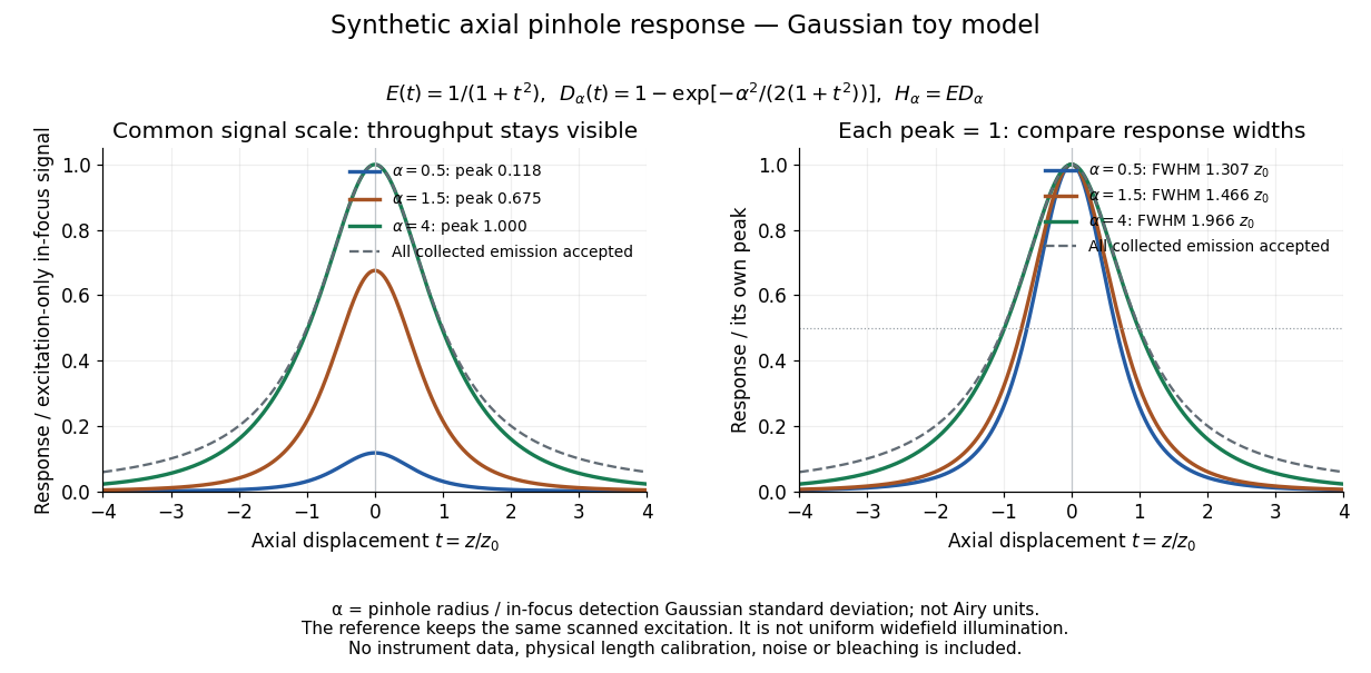
Synthetic axial response: narrower pinholes reduce throughput and suppress defocus
. Original Gaussian toy model, not measurements. The left panel keeps a common signal scale; the right divides each response by its own peak to compare widths. Here is a radius in units of detection-plane Gaussian standard deviation, not an Airy-unit diameter. The dashed reference is the same scanned excitation with all collected emission accepted, not conventional uniform widefield illumination. Both panels retain nonzero out-of-focus tails. Details.
For a vanishingly small pinhole, the peak-normalized synthetic response tends to , whose full width at half maximum is . With all collected emission accepted it tends to , of width . Meanwhile as the pinhole closes. The narrower normalized curve therefore accompanies a vanishing detected signal; peak normalization must not conceal that loss.
Confocal optical sectioning 2026-10-14
At one depth, scan the illumination spot across and and assign the detector reading during each dwell interval to a pixel. Move the specimen or objective optical lens axially to acquire the next depth. A stack of these optical sections samples three-dimensional structure. With beam scanning, the returning fluorescence commonly retraces the scanning optics: this descanning holds the image of the currently illuminated point at the detection pinhole. With stage scanning, the fixed spot and pinhole remain aligned while the specimen moves. [ref]
An optical section is a depth-weighted image of an intact specimen, with a finite axial response and tails. A physical cut actually separates a slice of material; its thickness and cutting damage are properties of the preparation. Changing optical focus selects another optical section without removing a slice, although illumination can still damage a specimen. Neither a thin physical slice nor a sharply displayed optical section makes the imaging point spread function infinitely narrow. [ref]
Introductory Confocal Concepts by Nikon Instruments Inc.. Fig. 2 discussion: focused-light sections rather than physical sectioning
Point response and section thickness answer different questions. For a spatially uniform, very thin fluorescent sheet, its response versus axial displacement is proportional to the lateral integral of the three-dimensional confocal response,Consequently a trace through a single bead, , does not by itself give the sheet's optical-section thickness. State which object and which full width at half maximum are being measured. A smaller axial sampling step gives more samples of the same response, rather than automatically improving diffraction-limited resolution. [ref]
Confocal microscopy (chapter manuscript) by Brad Amos and others. Appendix §6, manuscript pp. 42–43: thin fluorescent sheet translated through focus
Conjugate pinholes in confocal microscopy Created 2026-10-14 Updated 2026-10-20
Two planes are optically conjugate when an optical lens system images one onto the other. In confocal microscopy, an illumination pinhole is imaged onto the selected specimen point, and that specimen point is imaged onto the detection pinhole. Thus the two apertures select corresponding positions in different planes; they need not occupy the same physical plane. Modern laser instruments can supply the illumination point with an optical fiber or a suitable focused laser mode instead of a separate metal illumination pinhole. [ref]
Confocal microscopy (chapter manuscript) by Brad Amos and others. Amos, McConnell and Wilson, Confocal microscopy, manuscript pp. 5, 7–8: conjugate foci, Fig. 3, fiber-delivered illumination
A fluorescent emitter at the selected optical focus forms a compact point spread function at the detection aperture. An emitter displaced axially produces a broadened spot there through defocus; a smaller fraction of its collected light passes. The emitter still exists and still emits photons. Rejected photons strike the opaque mask or other parts of the instrument instead of contributing to the accepted detector channel. Neither a finite pinhole nor diffraction makes the accepted out-of-focus contribution exactly zero.
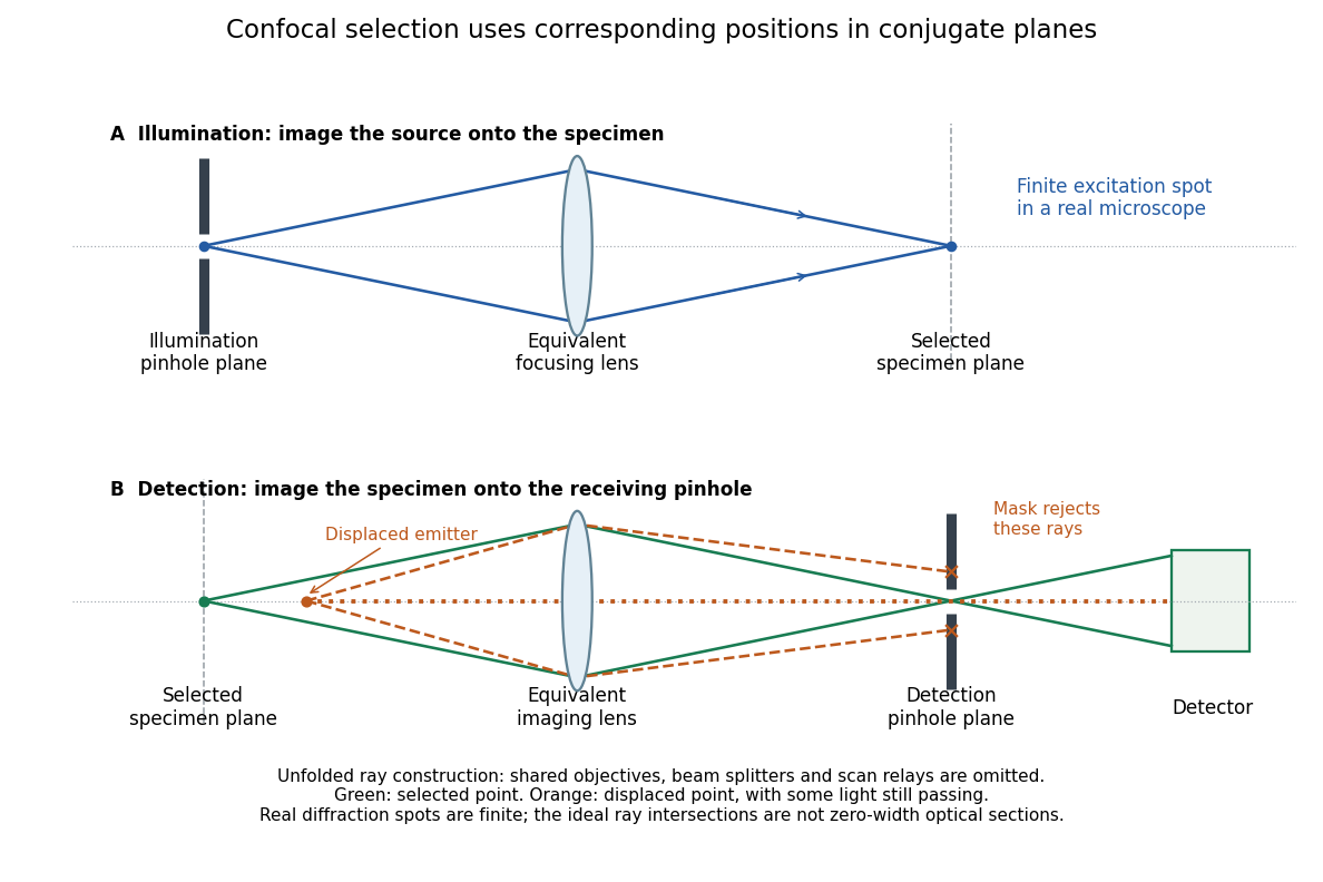
Conjugate illumination and detection pinholes in confocal microscopy
. Original unfolded geometrical optics schematic, not a scale drawing of an instrument. The top panel images an illumination pinhole onto the specimen; the lower panel images the selected specimen point onto the detection pinhole. Dashed orange light rays from an axially displaced point strike the mask, while an axial orange light ray passes. Real spots have finite point spread functions through diffraction; the drawing's perfect green intersection is only a ray construction. A fluorescence instrument may fold both paths through the same objective optical lens using a wavelength-selective beam splitter. Details.
The cone on the even integers is nonempty and Ellentuck topology open, while it is closed and nowhere dense in the ordinary topology on infinite subsets. Choose a finite-symmetric-difference parity colouring on that cone and take one colour class. The class is still ordinarily nowhere dense because its closure lies in the cone, but every stem-free refinement inside the cone meets both colours. Hence it is not completely Ramsey.
Face of a polyhedral cone 2026-10-14
A face of a polyhedral cone is for a linear functional nonnegative on . Every convex face of a polyhedral cone is exposed in this way. Faces include the whole cone and its lineality space, and are closed under intersection.
// Target: geometry-and-topology.bigb
For square-integrable and nested information , let and . The predictor is also -measurable, so the conditional variance error identity givesMore information cannot increase the average best squared prediction error. Equality holds exactly when the two conditional means agree almost surely; additional information can change the conditional distribution without changing its mean.
This is an averaged statement. Take with equal probabilities, and learn only whether is zero. The unconditional variance is . In the nonzero group, the conditional variance is , which is larger; in the zero group it is zero. Their weighted average remains . Both groups have conditional mean zero, so the extra information has not improved squared-error prediction, even though it has revealed whether the outcome is extreme or central. An individual group's conditional variance need not decrease.
Conditioning on a sum can create dependence 2026-10-14
Let be independent random variables, each with a Bernoulli distribution of parameter , and put . Unconditionally, the four ordered pairs each have probability . On the event , only and remain, each with conditional probability . ThusKnowing that exactly one trial succeeded makes observing one outcome informative about the other. This violates conditional independence given , even though the original random variables are independent. Given or , both variables are constant random variables and are conditionally independent there; that does not repair the failure at , an event of positive probability.
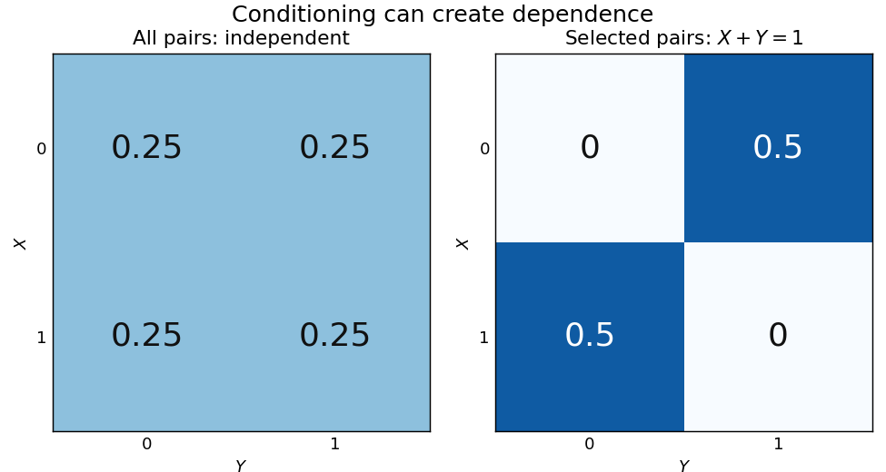
Selecting pairs with exactly one success makes independent trials dependent
. Left: four equally probable outcomes of independent fair Bernoulli trials. The selection retains exactly two pairs. Right: their conditional joint table has zero mass on the diagonal and off it. Within this selected model the conditional covariance is ; the two conditional marginal distributions remain fair. Details.
The conditional covariance here is . Both conditional variances are , so the conditional correlation coefficient is : within the selected group, . These conclusions follow from restricting a finite sample space, without positing any physical interaction between the trials.
This example and the shared-environment example establish both logical directions: independent random variables need not be conditionally independent, and conditionally independent variables need not be independent. When is represented as the joint result of two inputs in a causal directed acyclic graph, conditioning on it has the collider structure associated with collider bias. A probability calculation by itself establishes a dependence relation, not a physical causal mechanism or an intervention.
Conditioning can destroy independence 2026-10-14
Return to pairwise independence does not imply joint independence, where are independent fair bits and is their exclusive or. Given , only and remain, each with conditional probability . Given , only and remain, again each with conditional probability . Consequently,The conditional marginal distributions are still fair, so their product has four entries in either case. The actual tables differ: given , and given . Thus unconditional independence need not survive conditioning. Observing whether two bits agree restricts their possible combinations; no physical interaction between the original trials is required to produce that information constraint.
There are unlisted articles, also show them or only show them.