
Contradiction Created 2026-10-14 Updated 2026-10-25
A contradiction is an assertion or collection of assumptions from which logical falsity follows. Deriving both a statement and its logical negation is a standard example. A contradiction under a temporary assumption can establish that assumption's negation; classical proof by contradiction additionally uses this to establish positive conclusions.
Grouped proportional-hazards model 2026-10-14
When event times are observed only in intervals and the covariate vector is constant within an interval, a proportional hazards model gives . Thus the interval event probability has a complementary log-log link, with an interval-specific intercept. The person-period Bernoulli likelihood models several events in one interval directly, without inventing their order. It needs appropriate independent censoring assumptions and a consistent account of interval entry and observation.
Baseline survival function 2026-10-14
In a proportional hazards model , the baseline survival function is , corresponding to the reference covariate vector . Integrating the hazard function gives . Estimated hazard ratios alone therefore do not determine absolute survival probabilities: the baseline hazard or baseline survival function must also be estimated.
Inactive routes in proportional fairness 2026-10-14
When a route has zero active flows, its term is absent from weighted logarithmic utility. Its aggregate allocation is taken to be zero; a per-flow rate on it has no operational meaning and need not be uniquely determined. One must not divide by its zero population. Empty-network and empty-group cases can therefore be treated separately while preserving uniqueness of active-flow rates.
Dirichlet domain 2026-10-14
For a group of isometries acting properly discontinuously on the hyperbolic plane, and a point with trivial point stabilizer, the closed Dirichlet domain isIt is the intersection of the closed half-planes bounded by perpendicular bisectors between and its other group orbit points. The group orbit is locally finite and the hyperbolic plane is a proper metric space, so every point has a nearest group orbit point. This shows that the translates of cover the plane. Distinct interiors are disjoint, since being strictly closer to two different group orbit points is impossible. Boundary ties are allowed in the closed domain. Thus it is a geometric fundamental region.
Horseshoe lemma 2026-10-14
For a short exact sequence of modules with projective resolutions of its outer terms, there is a projective resolution of the middle term forming a degreewise split short exact sequence of resolutions. Lift the degree-zero projective cover of the quotient into the middle module and add the projective cover of the submodule; this surjects onto the middle module. Its kernel fits into the corresponding short exact sequence of kernels. Repeating this construction proves the claim. Additive contravariant functors preserve the degreewise split exact sequences with their direction reversed.
A finitely generated module over a Noetherian ring admits a possibly infinite free resolution whose every term is finitely generated. Surject a finite free module onto it; the kernel is finitely generated because a finite free module is Noetherian. Repeat this construction on the successive kernels. If the original module has finite projective dimension , its th syzygy is projective by dimension shifting of the Ext functor, giving a length- resolution with finite projective terms.
Completeness forces orthogonality of measurement projections Created 2026-10-14 Updated 2026-10-20
Let self-adjoint orthogonal projections sum to the identity. For in the range of ,The th term already equals , so for every . Hence and the projective measurement operators commute.
// Target: quantum-theory.bigb
Plane quartic with exactly two nodes 2026-10-14
Over the complex numbers the displayed projective plane curve has precisely two singular points, and . At either, with , , , the leading quadratic term is , so they are ordinary double points. The derivative equations in the chart have no solution: writing forces both and . The Bézout theorem proves irreducibility, since a factorization into degrees would require at least three intersections, whereas the only possible component intersections are the two transverse ordinary double points.
Quadric (algebraic geometry) 2026-10-14
A projective hypersurface defined by a nonzero homogeneous quadratic form. Over , diagonalization identifies its rank; it is smooth when the rank is and otherwise is a cone with a linear vertex.
Plane section 2026-10-14
The scheme-theoretic intersection of a projective hypersurface with a projective plane. If the plane is not contained in the hypersurface, restricting the defining homogeneous polynomial gives a projective plane curve of the same degree, with possible repeated components.
Sample space Created 2026-10-14 Updated 2026-10-14
The sample space is the set of outcomes represented by a probability model. One elementary outcome specifies a complete result at the level of detail the model keeps. An event is a subset belonging to the model's sigma-algebra ; it occurs when the actual outcome lies in that subset. Together with a probability measure , these form a probability space , with .[ref]
Introduction to Probability, Statistics, and Random Processes by Hossein Pishro-Nik. §1.3.1 Random Experiments: definitions of outcome, sample space, and event; three-toss example
Choosing a sample space means deciding which distinctions matter. For two tosses, recording the ordered head-or-tail sequence distinguishes from ; recording only the number of heads merges them. Neither representation is automatically wrong, but the second cannot answer a question about which toss was heads. Keeping a detailed sample space and defining a random variable for the desired observation lets several questions share one model.
A sample space alone assigns no probabilities. Even writing as a Cartesian product does not establish independence: that requires a condition on the probability measure. On a finite sample space with all subsets admitted as events,Only when all elementary probabilities are equal does this become , where the bars denote cardinality. This is the uniform distribution on a finite set, an additional modelling choice.
Sample spaces can also be infinite. For example, take , its Borel sigma-algebra, and the continuous uniform distribution. Then for , so each singleton has probability zero while . Thus an elementary outcome need not carry positive probability, and a continuous model cannot be understood by counting equally likely points. The distinction is developed in zero-probability event and countable additivity.
Product probability space 2026-10-14
For finitely many probability spaces , their product probability space has underlying set , the product sigma-algebra and product measure . The coordinate projections are jointly independent: for measurable , the probability of all coordinate conditions is . Conversely a family of independent coordinates has this product joint distribution. Product structure permits coordinate exposure and independent resampling in concentration arguments.
Sampling without replacement Created 2026-10-14 Updated 2026-10-14
Sampling without replacement selects distinct labelled units: after a unit is selected it is unavailable for the remaining draws. Distinct labels can carry equal numerical values, so repeated values do not necessarily imply a repeated unit. The rule alone does not specify selection probabilities; a procedure favoring particular units is still sampling without replacement but need not be simple random sampling.
In uniform sequential sampling without replacement, the next label is chosen uniformly among those remaining. For a population of labels, any ordered sequence of distinct labels has probability . Each size- subset has possible orders, so its probability is . This gives the fixed-size simple random sampling design. Equivalently, take the first labels of a uniformly random permutation. Restricting a uniformly random permutation to a specified label set preserves uniformity; biased modulo mappings should not replace uniform selection.
The draw positions have identical marginal probability distributions, but exhibit statistical dependence. If the first label is , the conditional probability that the second label is is zero, whereas its marginal probability is . Thus these draws are not independent and identically distributed when and . For a marked subset of labels, counting size- subsets with binomial coefficients gives the hypergeometric distribution. The resulting negative covariance explains the finite population correction for both counts and sample means.
Boole's inequality 2026-10-14
Boole's inequality, also called the union bound, bounds the probability that at least one of several events occurs by adding their individual probabilities. For a finite or countable family of events in the same probability space,The union includes outcomes where several events occur together. There is no independence assumption: adding the individual probabilities counts such outcomes repeatedly, which can only make the sum larger. The cap at one uses the total mass of a probability measure. For infinitely many events, the sum is a nonnegative series, possibly infinite; an infinite sum gives only the bound one. This is countable subadditivity of a measure specialized to a probability measure. See Probability: Theory and Examples (fifth edition) by Rick Durrett (Section 1.1, Theorem 1.1.1(ii), printed p. 2).
For example, choose uniformly from the twelve outcomes , using the discrete uniform distribution. Put . If , these are disjoint events and their union has probability , exactly the union bound. If , the union has only six outcomes, so its exact probability is , although both individual probabilities are still and the bound is still . If , the exact probability falls to with the same bound. These examples isolate overlap in the union bound by keeping the individual probabilities fixed.
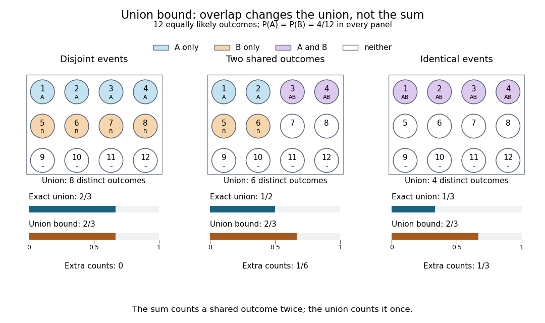
The same individual event probabilities give different exact union probabilities as overlap increases
. Each panel is a fully specified discrete uniform distribution on twelve numbered outcomes. Blue means only, orange means only, purple means their intersection, and white means neither. The bottom bars compare the exact union probability with the sum of the individual probabilities. The three unions contain eight, six, and four outcomes; the sum counts eight in every panel. Details.
The union bound is useful when each event is easy to control but their joint behavior is difficult to determine. A short proof uses indicator functions: at every outcome,Taking expected values and using linearity of expectation proves the finite bound.[ref] For a countable family, the finite unions increase to the full union; continuity of probability passes the finite inequalities to the limit. The closure of a sigma-algebra under countable unions ensures that this limiting union is an event. For the continuity of probability step, see Probability: Theory and Examples (fifth edition) by Rick Durrett (Section 1.1, Theorem 1.1.1(iii), printed p. 2).
Markov's inequality 2026-10-14
For a nonnegative random variable and threshold , Markov's inequality givesThe useful case has finite expected value; an infinite right side gives no finite information. The bound also holds if is nonnegative almost surely. Combining it with the elementary bound one gives . Nonnegativity is essential: negative values could otherwise cancel the contribution of large positive values to the expected value.
The idea is an average budget. Every outcome where contributes at least times its probability to , and the other outcomes contribute nonnegative amounts. Formally, the indicator function gives ; taking the expected value proves the bound. [ref]
https://ocw.mit.edu/courses/18-175-theory-of-probability-spring-2014/887e96172e82a615dac16fb26702d88b_MIT18_175S14_Lecture8.pdf. Sheffield, MIT 18.175, lecture 8: the expectation argument
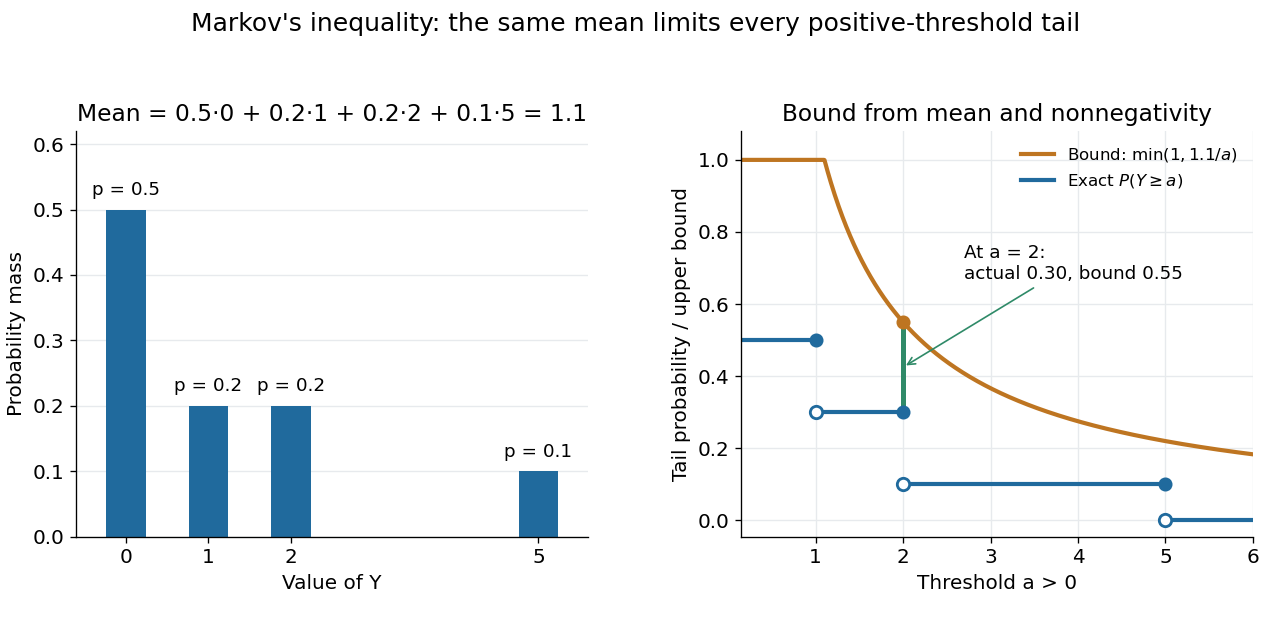
.For example, let take , , , with respective probabilities , , , . Its expected value is . At , the tail probability is , while the bound is . At , the tail probability is , while the bound is . A different probability distribution with the same expected value, putting masses and at and , attains the bound exactly at .

Markov's inequality is useful when a moment is easy to compute but a full probability distribution is difficult to determine. A nonnegative count with expected value less than one must have some positive probability of being zero, giving the first moment method. Applying the same bound to a squared centered random variable gives Chebyshev's inequality. Applying it to an exponential function of a random variable gives an exponential Markov bound, which can exploit more than a single moment.
Chebyshev's inequality 2026-10-14
For a real random variable with finite variance , expected value , and a threshold , Chebyshev's inequality givesOne can also cap this upper bound at one, since a probability cannot exceed one. If , taking gives . For example, at least of the probability lies strictly within two standard deviations of the mean. This statement needs only the finite variance assumption. If the variance is zero, almost surely and every positive deviation threshold has zero tail probability.
Consider a random variable uniformly distributed on . Its expected value is zero and its variance is . At the actual tail probability is , while Chebyshev's inequality gives . At the actual tail probability is zero, while the bound is . A valid bound need not describe the exact shape or bounded support of a particular probability distribution.
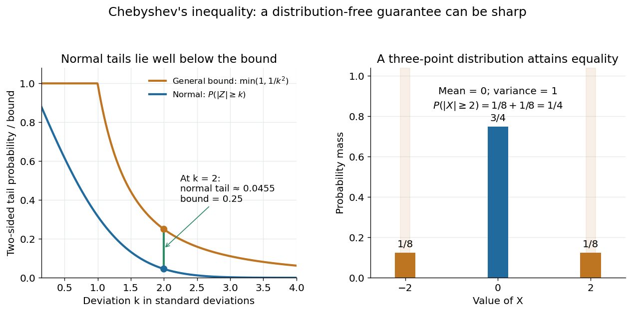

For the standard normal distribution, the actual tail probabilities beyond two and three standard deviations are approximately and , whereas the general bounds are and . More knowledge of the probability distribution can therefore improve the estimate. The comparison does not diminish the guarantee: the three-point example in equality in Chebyshev's inequality attains it exactly.
The proof is a one-line use of Markov's inequality on the nonnegative random variable . The event equals , and . This explains why the denominator is squared and why a finite variance supplies the necessary information. [ref]
https://ocw.mit.edu/courses/18-175-theory-of-probability-spring-2014/887e96172e82a615dac16fb26702d88b_MIT18_175S14_Lecture8.pdf. Scott Sheffield, MIT 18.175, lecture 8: Markov and Chebyshev bounds
.One important use is control of a sample mean. For independent and identically distributed random variables with finite variance , the variance of a sample mean is . HenceFor every fixed tolerance, the bound tends to zero as the sample size grows, proving the finite-variance case of the weak law of large numbers. For and , makes the bound . This is a sufficient bound under the stated assumptions, rather than an optimal required sample size.
An early historical source is Pafnuty Chebyshev's 1867 paper “Des valeurs moyennes”, published in French translation by N. de Khanikof. Its opening theorem bounds deviations of sums using their expected values and second moments, linking averages with control of exceptional outcomes. [ref]
https://www.numdam.org/item/JMPA_1867_2_12__177_0.pdf. Chebyshev, Journal de mathématiques pures et appliquées, 2nd series 12, 177–184 (1867)
. Predictive distribution Created 2026-10-14 Updated 2026-11-05
A probability law for a future observation conditional on currently available information. A posterior predictive distribution integrates the observation model over the posterior distribution of unknown parameters; a plug-in predictive law instead fixes an estimate of those parameters.
Infinite divisibility (probability) Created 2026-10-14 Updated 2026-11-05
A probability distribution is infinitely divisible if, for every positive integer , it is the distribution of a sum of independent and identically distributed random variables. Their common distribution may depend on . A normal distribution has this property by dividing its mean and variance by ; a Poisson distribution has it by dividing its rate. The unit-time law of a Lévy process is infinitely divisible because it is the sum of its increments on equal time intervals.
Heavy-tailed distribution Created 2026-10-14 Updated 2026-11-05
In the right-tail convention, every positive exponential moment is infinite. This is a tail property, not the assertion that the variance or all power moments must be infinite. A heavy-tailed subexponential distribution has the additional property that a sum's far tail is dominated by one large summand.
There are unlisted articles, also show them or only show them.