
Writhe 2026-10-14
For an oriented closed curve, geometric writhe is the signed crossing number averaged over generic viewing directions. For an individual link diagram, writhe of a link diagram is its signed crossing sum. Both depend on geometry or projection rather than only the link isotopy class.
Borromean rings 2026-10-14
The Borromean rings are a three-component link whose components are unknotted, which is nontrivial although removing any one component leaves an unlink. Its complement has a complete finite-volume hyperbolic three-manifold structure obtained from two regular ideal octahedra.
Split link 2026-10-14
A split link admits an embedded sphere in its complement with nonempty portions of the link on both sides. A split diagram admits a simple closed curve in the projection sphere separating nonempty portions of the diagram. A split diagram always represents a split link; the converse need not hold for an arbitrary diagram.
Link invariant 2026-10-14
A link invariant assigns the same value to links related by link isotopy. The Jones polynomial applies to oriented links, while its bracket precursor retains a framing dependence. An invariant need not distinguish all link types.
Isotropic-to-areal weak-field radius change 2026-10-14
The area of a symmetry sphere in the weak-field isotropic metric is . Equating it to defines the areal radius and gives the displayed change. To first order , and replacing by changes the perturbation only at second order. This explains why the isotropic angular correction disappears in the linearized Schwarzschild metric without discarding spatial curvature.
Weak-field photon-orbit validity 2026-10-14
The first-order null-orbit equation formally has a circular solution at , with . Its second-order equation gives a perturbation , hence instability. However, is outside the weak-field expansion. The exact Schwarzschild spacetime has a corresponding unstable photon sphere, but that physical result needs the exact geometry; extrapolating the linearized metric is not a controlled proof.
Parallel photon beams in linearized gravity Created 2026-10-14 Updated 2026-10-25
For signature and the curvature convention giving , take , and . A trace-free Lorenz-gauge particular solution has the displayed form. The vector is null, and , so co-propagating test photons are undeflected by this beam field. For a transversely uniform source, is one particular solution. A function of alone has vanishing wave operator and cannot source nonzero ; homogeneous gravitational perturbations and boundary conditions remain separate data.
The effective boundary coefficient is . All its ingredients come from initial scattering and the Robin boundary condition. Genuine zeros produce pole data; common zeros in numerator and denominator can instead be removable. It is incorrect to assert absence of boundary poles for every real Robin parameter.
Finite-horizon Robin spectral elimination 2026-10-14
Here and . The difference follows algebraically from the half-line NLS global relation and the Robin symmetry. Multiplication by the spatial-temporal jump factor gives , decaying in the second quadrant for . A triangular analytic change of the Riemann-Hilbert problem removes this finite-horizon defect while retaining the reconstruction and transferring all genuine pole information to the known determinant. No unproved large-time decay of the boundary values is needed.
Functional-group conversion in step growth 2026-10-14
In a balanced bifunctional feed there are initially groups and groups. Define the functional-group conversion in step growth by : the reacted fraction of either group type. Each join consumes one of each. Therefore . In the eight- example, three joins give and four give . In the latter state only three of eight starting monomer molecules remain isolated: their disappearance fraction is , different from . Neither this group-based nor disappearance of isolated monomers is the incorporated-feed fraction in the ideal living polymerization count.
With unequal initial counts , this article always uses , the conversion of the limiting groups. The reacted fraction of groups is , where . The fraction of all initial functional groups consumed is . At nonzero conversion these three fractions coincide only at . Naming the measured group type prevents an apparently correct equation from using the wrong conversion.
Stiff equation 2026-10-14
A stiff differential equation contains rapidly decaying modes alongside much slower dynamics. An explicit method may then require a small step for stability even when accuracy only requires resolving the slow modes.
Euler method Created 2026-10-14 Updated 2026-10-20
The Euler method approximates an initial value problem , , by evaluating the derivative at the current point and moving along that tangent line for a time . With , its displayed update needs one evaluation of per step. This simple rule turns local slope information into a whole approximate trajectory. MIT's course notes derive it by dropping the second-order Taylor remainder.[ref]
Take , , whose exact solution is the exponential function . The Euler method givesAt , the first values are . At , five steps give , compared with . The result decays but is too small: absolute stability alone does not ensure accuracy. At , the first values are , and at five steps give , while the exact solution is about .
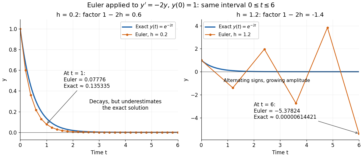

For the Dahlquist test equation , the Euler method has stability function with . Its absolute stability region is , the closed disk centred at with radius one. For the present real decay problem and , bounded numerical values require ; strict decay requires . At the values alternate without decay. These conditions follow directly from the amplification factor , matching MIT's criterion for .[ref]
https://web.mit.edu/10.001/Web/Course_Notes/Differential_Equations_Notes/node3.html. MIT 10.001, Forward and Backward Euler Methods, linear decay example
The Euler method is first order: with bounded second derivative and suitable Lipschitz continuity, its global error is on a fixed interval. In this example the logarithm gives for small positive . At , this means . It explains both the downward bias and why halving the step roughly halves the error once is sufficiently small.
A-alpha stability 2026-10-14
A numerical time-stepping method is -stable if its absolute stability region contains the negative-axis sector , for . With a stability function , this requires throughout that sector. At , this is A-stability.
Strict linear stability domain 2026-10-14
The strict decay convention for a linear stability domain demands that every numerical mode tends to zero on the Dahlquist test equation. For a one-step stability function it requires ; for a multistep method it requires every amplification root to have modulus below one. This differs from a boundedness convention that allows simple unit-circle roots, and from mesh-uniform finite-time numerical stability. Cambridge numerical analysis notes use the decay convention. Explicitly specifying the convention is essential for methods with undamped modes.
Stability matrix 2026-10-14
For near an equilibrium point, the stability matrix is the Jacobian matrix of the vector field evaluated at that point. Perturbations obey to first order. Its eigenvalues determine linear growth and decay: strictly negative real parts imply local asymptotic stability, while a positive real part gives instability. Zero real parts require further analysis. The stability matrix of a renormalization-group fixed point applies this construction to beta-function flows.
Stability threshold of a discrete exponential predator-prey model Created 2026-10-14 Updated 2026-10-25
For and , with , the positive equilibrium is , . Its Jacobian has trace and determinant . The unit-disc root conditions reduce to . At the roots form a nonreal conjugate pair and cross the unit circle; their argument satisfies . The unique threshold lies between one and because increases strictly and at threshold.
Isotope shift of a linear rotor 2026-10-14
Changing an isotope changes a mass and therefore the moment of inertia. If the bond length is held fixed, and every corresponding transition shifts by the same fractional amount. This leading inverse-reduced mass scaling is also used in the more complete diatomic formulation.[ref]
1Σ-Ground State Molecules. §2a, equations (4)–(5): isotope dependence of rotational constants and reduced mass
For a deliberately stipulated carbon monoxide example, take , , , , for both isotopic forms, and . The integer masses are simplifying inputs, not accurate isotopic atomic masses; the shared bond length is an imposed model assumption. Calculation givesIn particular,The heavier form's calculated line is rather than , a decrease of about . These are model predictions from the stated inputs, not published measured frequencies. An isotope changes the spacing as well as the first line; the shift is not a fixed additive offset for the whole spectrum.
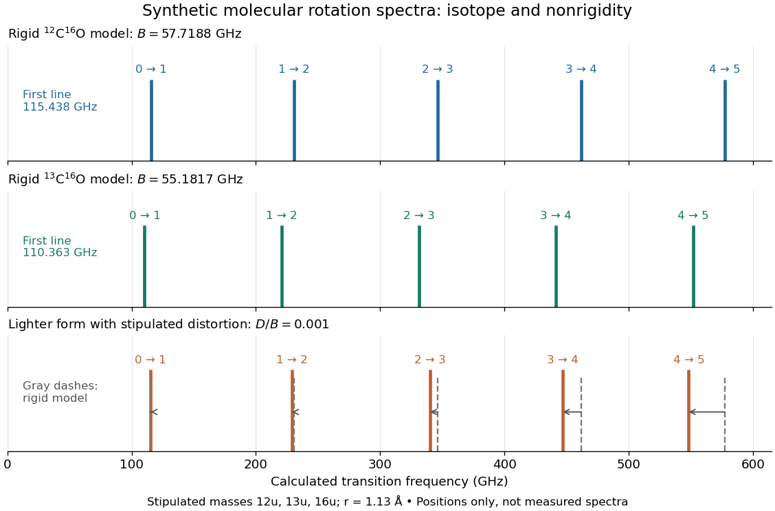
Synthetic rotational spectroscopy comparison: a heavier isotope compresses the rigid spectrum, while centrifugal distortion bends the spacing pattern
. Original equal-height sticks for through , using only the stipulated masses and bond length above. The lower panel additionally stipulates for the lighter form and compares with dashed rigid positions. Neither heights, distortion constant nor line frequencies are measured data; no thermal-population or instrument model is included. Details.
For the field-free, spin-free linear rigid rotor in one fixed internal quantum state, the electric-dipole interaction is . A nonzero permanent electric dipole moment along the molecular axis allows pure rotational photon absorption with and photon emission with . The matrix element between initial and final quantum states must be nonzero: the existence of an energy gap alone is insufficient. Relative to a chosen axis, polarization of an electromagnetic wave along selects ; transverse polarization of an electromagnetic wave permits .[ref]
Lecture 24 Supplement: Energy levels of a Rigid Rotor by Dudley Herschbach. printed pp. 2–3: dipole transition integrals, polarization and selection rules
Hydrogen chloride and carbon monoxide are examples with a permanent electric dipole moment. By symmetry, molecular hydrogen and carbon dioxide have no permanent electric dipole moment in the ideal symmetric internal state. They still rotate and have rotational energy eigenvalues, but the simple permanent-electric dipole spectrum described here is absent. This restriction concerns this interaction and these assumptions, not every possible way of detecting molecular rotation.
Rotational constant Created 2026-10-14 Updated 2026-10-18
In this article the rotational constant is a frequency,Its dimensions are , since the Planck constant has dimensions and a moment of inertia has dimensions . Some authors instead call the energy-valued rotational constant; this is the convention in the earlier synthetic molecular beam electric resonance diagram. A third convention uses the spectroscopic wavenumber , with the speed of light. Always check units before using .
If is known and the two masses are specified, the rigid two-atom model gives the bond length . This is why rotational spectroscopy can constrain molecular geometry. A real fitted constant can depend on molecular vibration, so this inference alone does not establish an equilibrium bond length.
Dual feasibility 2026-10-14
For minimization with constraints , , a dual-feasible vector obeys , so is a lower bound on every primal-feasible objective value. For a simplex dictionary with basis matrix , the associated vector is . Its basic reduced costs are zero and its nonbasic reduced costs are . Thus nonnegative reduced costs are exactly dual feasibility in this minimization convention; basic primal values may still be negative, as in the dual simplex algorithm.
There are unlisted articles, also show them or only show them.