
Grid-separated additive coordinates 2026-10-14
For five pairs of continuous functions on , one can arrange that at every arbitrarily fine scale there are closed interval families whose product rectangles cover each point at least three times, and within each family the images under are mutually disjoint. To see this, put gaps near five shifted fine grids; gap sets for different shifts are disjoint. Each coordinate misses at most one family, so a pair misses at most two. Approximate any prescribed pair of functions by constants on the complementary intervals, interpolating across gaps. Perturb the finitely many constants to avoid all equalities between distinct pair sums. The rectangle images are then separated by a positive distance, a property preserved under sufficiently small uniform perturbations. For each required mesh size this property defines a dense open subset of . The Baire category theorem gives a tuple satisfying every scale simultaneously.
For , choose a positive continuous function with for . Such an is obtained by piecewise linear interpolation of a sufficiently large increasing sequence. Then tends uniformly to zero at infinity. Transport to by and extend it by zero on the boundary; the extension is continuous. Apply the compact Kolmogorov-Arnold representation theorem, then multiply by . Multiplication introduces no additional primitive operation because uses only addition and continuous one-variable squaring and scaling.
Möbius invariance of on-shell closed-string vertex integrals Created 2026-10-14 Updated 2026-11-05
Under with , the coordinate measure contributes at insertion . The Koba-Nielsen factor contributes . Four-momentum conservation makes this exponent , so the factors cancel precisely on the displayed tachyon mass shell. The correlator alone is covariant; its product with all the coordinate measures is invariant.
Rarefied gas flow approximations 2026-10-14
For , frequent gas–gas collisions can establish a local Maxwellian before macroscopic conditions change appreciably. Under this additional near-equilibrium assumption, the hydrodynamic limit of the Boltzmann equation motivates a continuum approximation with Navier-Stokes equations and heat conduction. A no-slip boundary condition is a leading wall approximation, not a statement about individual molecular velocities.
With a small but finite Knudsen number, a useful slip approximation retains continuum bulk equations and corrects wall velocity and temperature. A Navier slip boundary condition can represent the leading tangential velocity correction, but its slip length must come from the relevant gas–wall interaction model. A nearby Knudsen layer still requires kinetic treatment if its detailed structure is wanted. Slip corrections are perturbations; extending them into order-one Knudsen numbers has no general accuracy guarantee. At order-one Knudsen number, wall and intermolecular collisions both matter; this transitional situation calls for a kinetic theory model. At , free molecular flow becomes a useful limiting approximation. These are scale comparisons, with accuracy depending on geometry, flow conditions and the observable, rather than universal sharp numerical boundaries. [ref]
https://ntrs.nasa.gov/api/citations/19860015045/downloads/19860015045.pdf#page=3. Frank G. Collins (1985), Low Density Gas Dynamic Wall Boundary Conditions, introduction
Clean subset superposition preparation 2026-10-14
Suppose a known list of distinct -bit strings is available and computational basis transpositions on qubits have polynomial-size implementations. Start with the uniform superposition state of index labels , leaving the data zero. First swap with for each nonzero . Next, for each , swap with . Distinct index labels separate the first-stage pairs, and distinct data strings separate the second-stage pairs. Thus no later transposition disturbs an earlier term. At most transpositions prepare the uniform data state and return the quantum ancilla to zero. For the quantum circuit has polynomial size. This assumes the list is available; a membership predicate alone does not supply it.
Alternating knot 2026-10-14
An alternating knot is a knot admitting an alternating knot diagram. A nonalternating diagram can still represent an alternating knot; the property of the knot is existential over its diagrams.
The matrix in the Knill--Laflamme condition is positive semidefinite, since is the squared norm of for any normalized code state. Diagonalizing it gives linear combinations with . For , is an isometry of the code into an error-image subspace, and these subspaces are orthogonal. Measuring their projectors and applying recovers the logical state. Complete the operation arbitrarily on the orthogonal complement to obtain a quantum channel. This construction corrects every noise map whose Kraus operators lie in the specified error span, including coherent superpositions of error operators.
Necessity of the Knill-Laflamme condition 2026-10-14
If a common recovery quantum channel with Kraus operators restores every pure code state after each error , then each vector is parallel to . Linearity on basis vectors and their pairwise superpositions forces , with the scalar independent of the logical state. Insert between two error operators to obtain the displayed Knill--Laflamme condition. This proves necessity without presuming an orthogonal syndrome description of recovery.
Invariant-normalized scalar mode extraction Created 2026-10-14 Updated 2026-10-20
For a free real scalar field expanded with measure and , the displayed Klein-Gordon inner product extracts its annihilation operator. Indeed and ; spatial Fourier inversion removes the measure. Taking the Hermitian adjoint gives . The equal-time canonical commutation relation then gives .
Density-weighted mean kinematic viscosity Created 2026-10-14 Updated 2026-10-20
For a vertically stratified accretion disk with surface density , the density-weighted mean kinematic viscosity is . In an alpha disk with , this becomes .
// Target: astrophysics.bigb
Dimension bound for Killing vector fields 2026-10-14
On a connected -dimensional pseudo-Riemannian manifold, evaluation of a Killing vector field and its first derivative is injective by Killing transport. The value has components and the Killing equation makes the derivative an antisymmetric two-tensor with components. Their sum gives the bound. Flat metrics attain it through with . Connectedness is essential for a uniform global bound in terms of : independent fields can be supported on different connected components.
Parallel-spinor classification of vacuum four-geometries Created 2026-10-14 Updated 2026-11-05
A parallel commuting Dirac current is causal. If timelike, the geometry locally splits as a time line times a three-dimensional Ricci-flat metric; three-dimensional Ricci flatness implies flatness. If null, the stabilizer of a parallel spinor in contains only null rotations, and the local vacuum metric is with . Constant spinors obeying are parallel. These are local statements; global quotients must preserve a compatible spin structure.
Anti-de Sitter Killing-spinor connection Created 2026-10-14 Updated 2026-11-05
For constant sectional curvature , spin curvature is . The added Clifford term in has the opposite commutator, making flat. On a simply connected region, parallel transport of any initial spinor is path independent and constructs solutions of . Thus Anti-de Sitter spacetime and its universal cover admit the associated Killing spinors locally and, with appropriate global spin data, globally.
Bifurcate Killing horizon 2026-10-14
A bifurcate Killing horizon consists of two intersecting null Killing horizons of the same Killing vector field, which vanishes on their spacelike intersection, the bifurcation surface. In regular Kruskal coordinates the horizons are and , and their intersection is . The displayed field is tangent and normal to each horizon branch and zero on the intersection.
Horizon angular velocity 2026-10-14
In an axisymmetric stationary spacetime, the horizon angular velocity is the constant coefficient in the null horizon generator , where is the stationary Killing vector normalized at infinity and generates axial orbits with period . It measures rotation relative to the stationary frame at infinity. For a Kerr black hole, . It enters the rotating physical-process first law through the horizon flux of .
Kerr-Newman horizon temperature 2026-10-14
The outer-horizon surface gravity is . Hawking radiation or nondegenerate Euclidean black-hole regularity condition gives in units . The zero-temperature extremal value is the nonextremal limit; conical regularity alone does not fix a Euclidean period at a degenerate horizon.
First law for the Kerr-Newman family 2026-10-14
Differentiate , and . Eliminating and gives the displayed relation, with and . Matching Hawking temperature to this First law of black-hole mechanics fixes the Bekenstein-Hawking entropy as .
Lense-Thirring precession 2026-10-14
Lense-Thirring precession is the rotation of orbital angular momentum caused by the gravitational field of a spinning mass. In the secular weak-field picture, the precession vector is parallel to the central spin. Thus an annulus has torque proportional to , perpendicular to . Summing such torques preserves this orthogonality even if their radial coefficients differ. Dissipation and the internal response of a warped accretion disk can supplement precession with an alignment torque.
Nullity of a linear map Created 2026-10-14 Updated 2026-11-05
The nullity of a linear map is , the dimension of its kernel. It counts independent input directions that can change without changing the output. For a finite-dimensional vector space , the rank-nullity theorem givesFor an matrix of matrix rank , this is , using the number of columns, not the number of rows. [ref]
Linear Algebra Done Right by Sheldon Axler (4th edition). Sheldon Axler, Linear Algebra Done Right, fourth edition, §3B, theorem 3.21: rank plus nullity equals the input dimension
The nullity answers a practical question about a linear system: once one input is known to produce the requested output, how much freedom remains? If , its fiber of a function over isIndeed, exactly when . Thus every nonempty fiber is an affine subspace of dimension , with the same direction space as the kernel. The kernel itself is the fiber over zero. Outputs outside the image of a linear map have empty fibers; the nullity does not guarantee existence, and we assign no solution-space dimension to an empty fiber here.
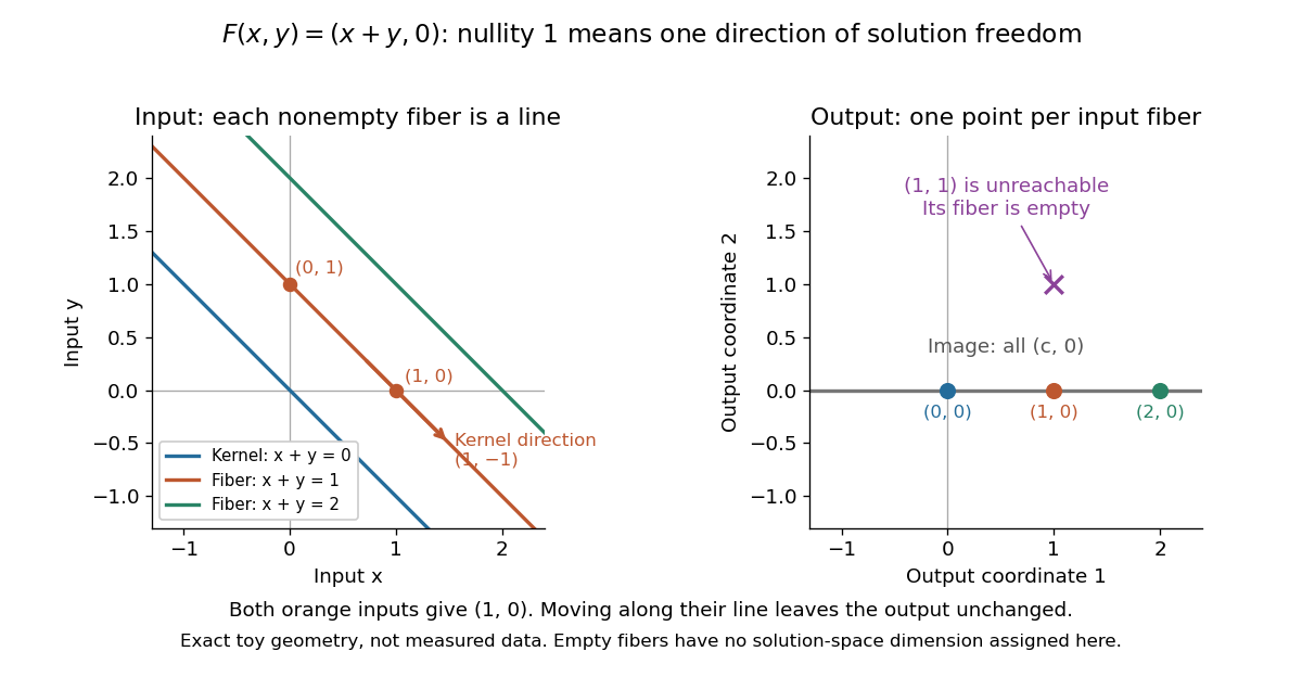
Nullity one gives parallel solution lines for
. Each colored input straight line is the fiber over the corresponding output . The blue line through the origin is the kernel. The orange inputs and give the same output; their difference belongs to the kernel. The output lies outside the image of a linear map and has no input. Exact toy geometry, not measured data. Details.
In the diagram, has matrix , matrix rank one and nullity one. Its kernel has basis , and the full solution of is . One free scalar moves the solution along a straight line; the output is impossible.
The existing three-input example instead has rank two and nullity one. Its image of a linear map is all of , andEvery output has a solution straight line. In contrast, has rank one and nullity two, with kernel basis . Its reachable output has the solution affine subspacea plane, while with has no solution. These two linear maps have the same input and output dimensions but different freedom and reachability. Computing the kernel separates what an output determines from what an extra constraint would have to fix. For either example, a basis of the kernel gives one independent free scalar per basis vector, which is why nullity measures freedom rather than the number of solutions.
Noninjective linear measurement 2026-10-14
When a measurement model is a linear map , its kernel records changes that its readout cannot distinguish. For example, the rectangular kernel and solution-fibre example measures only and . Even exact readouts leave the whole fiber possible. Repeating either readout with greater precision cannot distinguish those inputs: their outputs agree exactly. This ambiguity follows from a nontrivial kernel, rather than from measurement error.
Additional information can remove a null direction of a linear map. In that example, adding a third linear functional that reads distinguishes , because its third readout is . More generally, additional linear functionals give unique recovery of all inputs exactly whenThis follows by applying the trivial kernel criterion to the combined linear map . Merely adding repeated linear equations does not meet this condition. On a finite-dimensional input vector space, each added scalar readout can increase the matrix rank by at most one, so at least extra independent readouts are needed for recovery of unrestricted inputs.
Restrictions on the possible inputs can also make recovery unique. If the allowed inputs form a set , two allowed inputs are indistinguishable exactly when their difference is in the kernel. Thus is injective on precisely when no difference of distinct points of is a kernel vector. Such a restriction is extra information about the input; the original readout alone determines only its fiber.
There are unlisted articles, also show them or only show them.