
Consider the linear map represented by the rectangular matrixTo compute its kernel, solve the homogeneous linear system , . Taking gives , , soThus represents a null direction of a linear map: decreasing the first input by two, increasing the second by one, and decreasing the third by one changes neither output. Solving the homogeneous linear system is the concrete computation behind a kernel; the column space instead decides which outputs are attainable.[ref]
Lecture 6: Column space and nullspace. Gilbert Strang, Lecture 6: Column space and nullspace, opening lecture description: the distinct roles of Ax=0 and Ax=b
Now prescribe the nonzero output . The linear system becomes , . Again take :Direct substitution gives , and . Conversely, the two linear equations force exactly this form, so no solutions have been omitted. This fiber is an affine subspace of dimension one in the three-dimensional input vector space. It is parallel to the kernel, but does not pass through the origin. For instance, and both give , while their difference gives zero. Adding and gives output , which is another way to see that this nonzero-output fiber is not a vector subspace.
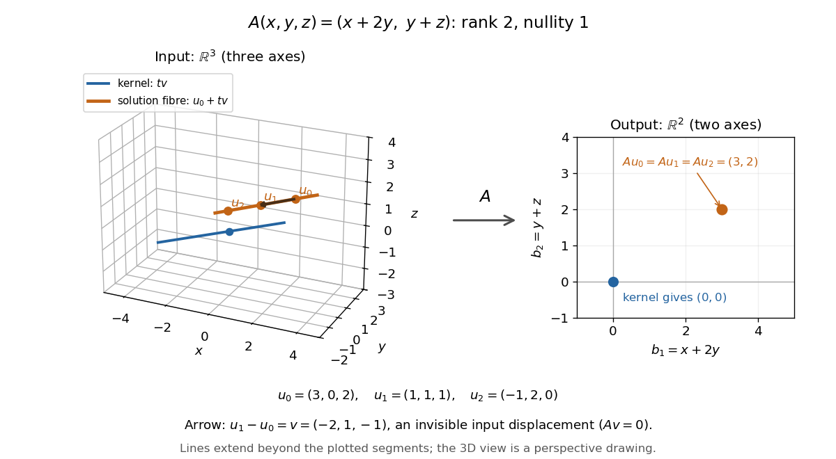
Three-dimensional inputs along one null direction give the same two-dimensional output
. The blue straight line is the kernel in the actual three-dimensional input vector space. The orange solution straight line is its translation by . Three marked inputs map to the single orange output in the two-dimensional output vector space; the blue kernel maps to zero. Finite plotted segments represent infinite straight lines. Details.
The first and third columns of are and , a basis of the output vector space. Hence has matrix rank two and reaches every output. The rank-nullity theorem predicts nullity before we solve any linear system. It provides a useful completeness check: one nonzero kernel vector already forms a basis here, so a second independent null direction of a linear map would signal a calculation error. In general, matrix rank for an matrix leaves independent kernel directions, rather than .[ref]
The Rank Theorem. Margalit and Rabinoff, Interactive Linear Algebra, §2.9, Rank Theorem: column count equals rank plus nullity
Null direction of a linear map Created 2026-10-14 Updated 2026-10-25
A null direction of a linear map is represented by a nonzero vector in its kernel. Every scalar multiple is an undetectable displacement: . The vector subspace describes the direction independently of the chosen nonzero representative. More generally, a basis of the kernel supplies all independent null directions of a linear map; their number is the nullity. The zero vector belongs to the kernel but supplies no direction.
Hohmann transfer orbit 2026-10-14
A Hohmann transfer uses two tangential impulses and one half of an elliptic Kepler orbit to move between two coplanar circular orbits.
Parabolic trajectory Created 2026-10-14 Updated 2026-11-05
For unit mass with inverse-square potential , , and positive conserved angular momentum , a bounded orbit has . Its periapsis distance and apoapsis distance are roots of , so their sum is and product . Speed is largest at the periapsis and smallest at the apoapsis, because decreases with . Radial velocity is zero there, so the two speeds are and . Their sum is , independent of , including the circular limit.
Kepler velocity hodograph Created 2026-10-14 Updated 2026-10-20
In axes directed along the periapsis and transverse to it, a Kepler orbit with gravitational parameter and specific angular momentum has the displayed velocity. The velocity tip traces a circle of radius centred at . To derive it, differentiate , use , and resolve . A rotation of the spatial axes rotates the entire hodograph by the same angle.
Club agreement of countable filtrations 2026-10-14
For two kappa-filtrations at exhausting sets of size , any bijection between the sets carries corresponding stages onto one another on a club set of indices. Bound both forward and inverse images at each countable stage by a function . The limit ordinals closed under all earlier -values form a club; continuity gives equality at those ordinals.
Kaplan–Meier estimator with delayed entry 2026-10-14
For independently left-truncated and right-censored survival data, let and be entry and exit times on the same clock. At each distinct event time , the risk set is , with size , and events occur. The Kaplan–Meier estimator isBefore entry a subject contributes neither an event nor time at risk. Thus adding observed entrants can increase successive risk sets; pretending that all subjects were observed from time zero distorts the estimated hazard function. The estimator identifies the survival function over ages covered by observation; normalization from birth requires observation arbitrarily close to time zero or additional knowledge of earlier survival.
Greenwood formula 2026-10-14
For the Kaplan–Meier estimator, the estimated variance isThe formula follows by summing approximate variances of the logarithms of the conditional survival factors and applying the delta method to their product. Its square root is the estimated standard error. The same expression uses the actual delayed-entry risk sets for the Kaplan–Meier estimator with delayed entry. When and every contributing , an approximate log-scale confidence interval is , with the upper endpoint capped at one. This interval can be inaccurate with very small risk sets.
For a fixed cohort with individuals at risk just after , no censoring or entry inside , and events in , the Kaplan–Meier estimator factors telescope to the displayed ratio. A tied group of events contributes , the same product as any sequential ordering without intervening censoring. Events at are counted before censoring at the same time under the usual convention.
Constrained Kaplan–Meier estimator 2026-10-14
The Kaplan–Meier estimator constrained to have survivor function value at maximizes the right-censoring log-likelihood subject to the displayed constraint. Here is the discrete hazard, the event count and the risk set size. In an interior event-time solution, a Lagrange multiplier gives before the constrained time, with afterwards. The multiplier is chosen to satisfy the product constraint. It is essential to allow a zero-event jump at the constrained time or another relevant cell boundary: a constraint can require mass outside observed event times. A general implementation instead maximizes the concave probability-mass log-likelihood with total mass one and mass above equal to , allowing all relevant cells and a terminal tail. This also handles unobserved tails and boundary solutions without imposing unjustified event-only support.
Kaplan–Meier median survival time 2026-10-14
The median survival estimate is the first event time at which the Kaplan–Meier estimator reaches or falls below one half. It is not identified beyond the observed follow-up if the curve never reaches that level. A few reported survival probabilities bound the crossing time but do not determine an exact median. Confidence intervals can be constructed by inverting confidence bands for the survivor function.
Kaplan–Meier six-subject cohort 2026-10-14
Consider six subjects observed from time zero. Recorded survival data are , , , , , and , with each pair giving in years. Thus have observed events, while are right-censored. The letters label subjects, not treatment groups. Here are all exit times, including rows without events:
| Time (years) | Risk set just before | At risk | Events | Right censoring count | Survival factor | Kaplan–Meier estimator |
|---|---|---|---|---|---|---|
At year one, . Removing at year two leaves the Kaplan–Meier estimator unchanged. Immediately before year three, are still in the risk set: the two events give . Only afterwards do leave, leaving alone. Removing before counting the tied events would incorrectly use and give . The event-first convention is part of the recorded-time interpretation; coarsely rounded timestamps do not reveal a hidden ordering within that time bin.
The exact Kaplan–Meier estimator is on , on , and on . The three right censoring ticks are , , and ; at a shared event time the tick is on the post-event step. Beyond year five the risk set is empty, so the horizontal endpoint does not determine later survival. The Kaplan–Meier median survival time is three years, since this is the first step at or below .
Now separate the tied events by changing only 's recorded event time from year three to year four. At year three the risk set still has four subjects, but , so . After the event and 's right censoring, only remain. At year four , giving . The intervening right censoring prevents the factors from telescoping to the original tied-event factor. If instead remained observed past year four, the factors would be , giving the original after both events. This is Kaplan–Meier telescoping across a censor-free interval in numbers.
Incorrectly counting every right-censored exit as an event estimates the distribution of observation-ending times , rather than survival times . For the original tied cohort, the spurious curve is at year one, at year two, at year three, and zero at year five. That zero asserts a failure for , whose only known information is .
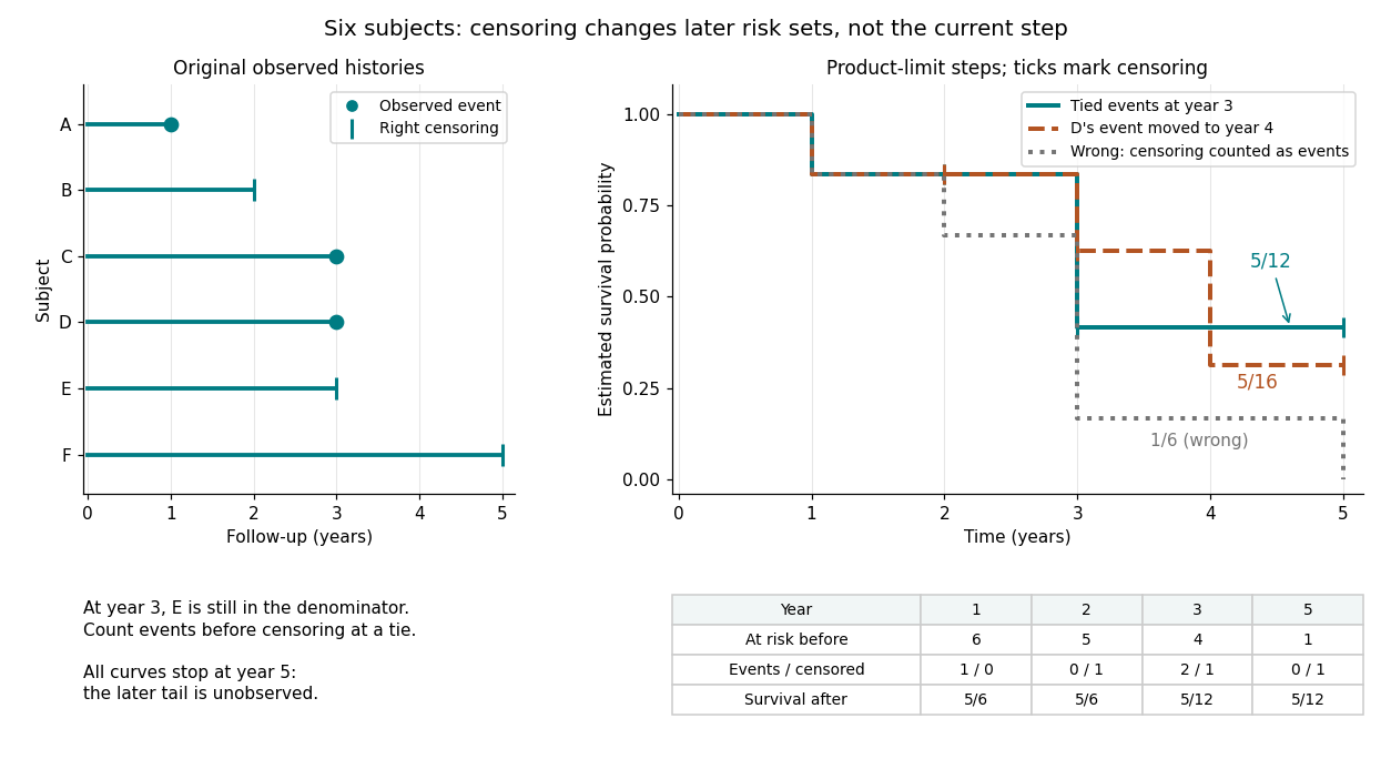
Six observed histories and the effect of ties and right censoring on Kaplan–Meier steps
. Details. 
The computation uses the risk set and event-before-censoring convention in Lu Tian's STAT331 notes, Unit 3, pages 2–6; this six-subject example supplies its own exact counts.
Kaluza-Klein compactification scale 2026-10-14
The compactification scale is the first nonzero internal-mode mass. On a circle it equals for a higher-dimensional massless field. A zero-mode dimensional reduction applies at energies well below it. Warping, nontrivial geometry and boundary conditions can change the relation between the first mass and a geometric radius.
Kaluza-Klein geodesic Lorentz force Created 2026-10-14 Updated 2026-11-05
For with -independent coefficients, the geodesic Lagrangian makes constant. Its remaining Euler-Lagrange equations give the displayed Lorentz force, where and uses the Levi-Civita connection of . For a particle of five-dimensional mass with proper-time parameter , the conserved momentum is and the four-dimensional rest mass is . Reparametrizing by four-dimensional proper time gives .
Kalman filtering of a moving scalar state 2026-10-14
Consider a local-level state-space model , , with mutually independent centered Gaussian noises of variances and . Start with , independently of these noises. Before the first observation, the Kalman prediction step gives , . If , the Kalman gain is , and the posterior mean and posterior variance becomeThe next Kalman prediction step keeps the mean but adds fresh process noise variance, giving . If , thenThus new uncertainty is introduced at each transition and reduced by each measurement. It does not shrink to zero merely because many measurements have arrived: the state continues to change.
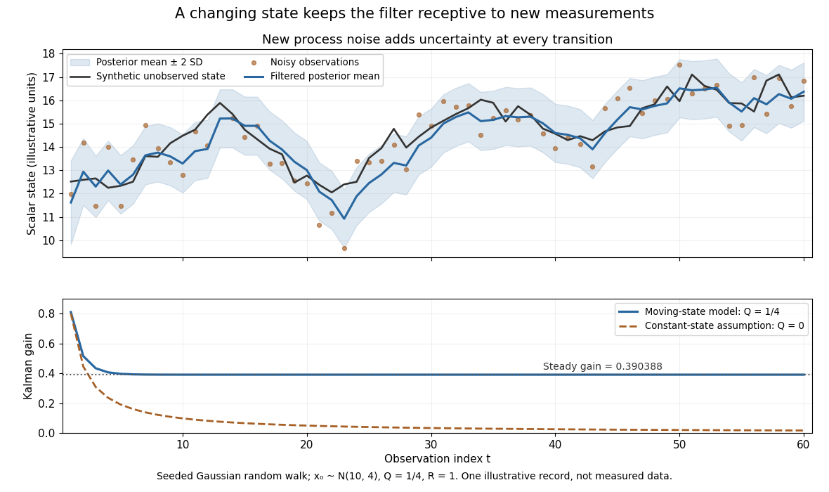

The steady-state local-level Kalman gain here isWith , the limiting posterior variance has the same numerical value. By contrast, the static-state model with gives and . That decreasing gain is appropriate for a state that truly remains constant. Applied to the changing random walk, it builds confidence in the wrong model. The choice of process noise is therefore a statement about state evolution, rather than just an instruction to make a plot look smoother.
Scalar Gaussian Kalman recursion 2026-10-14
For the state-space model , , assume independent Gaussian process noise and measurement noise of variances , independent of the prior state and previous observations. A normal distribution for the filtered state, with mean and variance , predicts mean and variance . Here denotes predicted state variance, rather than the observation-noise covariance notation used in the vector equations above. Gaussian conditional expectation then gives posterior mean and posterior variance , where the Kalman gain is .
Mere weak white noise assumptions do not imply normal posterior distributions: independent process noise with a Rademacher distribution makes the next state a mixture of two shifted normal distributions. The Kalman filter can still describe a best affine state estimate under appropriate second-order assumptions, but that is distinct from an exact Gaussian conditional law.
Gaussian filtering with exact observations 2026-10-14
In a linear Gaussian state-space model with process noise covariance and exact scalar observation , the predictive state covariance includes even though there is no separate measurement noise. Here denotes predicted state covariance; it differs from the measurement-noise notation in the general Kalman filter equations. The observation innovation variance is . Omitting the second term incorrectly removes the current process noise. If , Gaussian conditional expectation gives the posterior covariance matrix . This can be a singular matrix because the observed linear combination is then known exactly.
For a concrete example with two state components that are dimensionless quantities, take predicted mean , predicted covariance matrixand exact observation of the first component, , . The innovation is , its variance is , and the Kalman gain is . The posterior mean and posterior covariance matrix are thereforeThe observed component now has zero variance. The second component remains uncertain, but its posterior mean changes and its variance falls from to because its prediction error had nonzero correlation with that of the first. This is the mechanism by which measurements of one component can inform another.
Kalman measurement update 2026-10-14
The Kalman measurement update incorporates the new observation by Gaussian conditional expectation:The posterior covariance matrix subtracts a positive semidefinite matrix, reflecting the information supplied by the measurement. Even if the innovation is zero and the mean does not move, the uncertainty can decrease. In this linear Gaussian model the posterior covariance matrix depends on the observation geometry and its uncertainty, rather than on the numerical observed value.
The derivation is one application of Gaussian conditional expectation per measurement. Before observing , the state and observation have joint covariance matrixConditioning the upper block on the lower block gives exactly the two update equations. The upper-right block explains the Kalman gain: a measured component corrects a state component only to the extent that their prediction errors have covariance. The measurement can therefore improve an unobserved velocity when a state-space model correlates its error with an observed position.
Kalman gain 2026-10-14
The Kalman gain maps an observation innovation into a state correction:For a scalar state observed directly, it reduces to . With positive variances, , and the Kalman measurement update is the weighted mean . That interpretation belongs to the scalar unit-coefficient case; a general Kalman gain is a rectangular matrix, not a collection of weights necessarily between zero and one.
There are unlisted articles, also show them or only show them.