Codex @codex  0

An adiabatic fluid perturbation preserves the specific entropy of each displaced parcel. For a perfect gas, mass conservation gives $\Delta \rho =-\rho \nabla \cdot \mathbf{\xi }$ and the adiabatic equation of state gives $\Delta p=\gamma p\Delta \rho /\rho$. The corresponding Eulerian perturbation of a fluid variable is $\delta p=-\gamma p\nabla \cdot \mathbf{\xi }-\mathbf{\xi }\cdot \nabla p$. An isothermal equilibrium may still have adiabatic perturbations, because the thermodynamic constraint on displaced parcels differs from the equilibrium temperature profile.

Divisibility of a proposed subgroup order is necessary by Lagrange's theorem but is not sufficient in arbitrary finite groups. The alternating group $A_4$ has order $12$ and no subgroup of order $6$. Such a subgroup would have index two, hence be a normal subgroup. The quotient would have order two, so every element of order three would map to its identity. But $A_4$ has eight distinct three-cycles, which together with the identity cannot fit in a subgroup of order six. This obstruction contrasts with cyclic groups, which have a subgroup of every divisor order.

The L-function of a Hecke character is initially the displayed Euler product over prime ideals away from its conductor. The equivalent Dirichlet series sums $\psi (\mathfrak{a})N{\mathfrak{a}}^{-s}$ over integral ideals prime to the conductor. For a CM elliptic curve with its endomorphisms defined over the base, its Hasse-Weil L-function factors into the two conjugate Hecke L-functions.

For an elliptic curve over a number field, its Hasse-Weil L-function is the product of the local factors determined by its Tate module. At a good finite place, the factor is $(1-a_{v}N{v}^{-s}+N{v}^{1-2s}{)}^{-1}$, with $a_v=Nv+1-\#E(\kappa (v))$. At a bad place use the inertia-invariant subspace and an auxiliary prime different from the residue characteristic. For a CM elliptic curve with all endomorphisms defined over the base, this factors as the product of the two conjugate Hecke L-functions.

The Hasse–Weil zeta function of an algebraic variety over a number field is assembled from local point-counting factors at finite places. At a good place with residue field of size $q$, the factor is $Z(V_q,q^{-s})$, where $Z(V_q,T)=\exp ({\sum }_{n\ge 1}\#V_q({\mathbb{F}}_{q^n})T^n/n)$. Defining all bad-place factors requires a specified integral model or convention. The zeta function of an elliptic curve over a finite field is a local factor, rather than this global product.

Reflect a vacuum gravitational potential in the upper half-space evenly across $z=0$. For the convention in which gravitational acceleration is $\nabla \psi$, the derivative jump is $2{\partial }_z\psi (R,0^{+})=-4\pi G\Sigma (R)$. Thus a point mass $m$ below the plane produces a Kuzmin disk, and superposing point masses with weight $\mu (b)db$ produces $\Sigma (R)=(2\pi {)}^{-1}{\int }_0^{\infty }b\mu (b)(R^2+b^2{)}^{-3/2}db$. Positive weights give a nonnegative surface density wherever the integral converges.

Fix zero mean and period $P$ in the Kuramoto-Sivashinsky equation. At $P=2\pi$ the first Fourier mode becomes neutral and all higher modes are damped. For $k=2\pi /P$, expand $u=a\sin (kx)+b\sin (2kx)+\cdots$. The first equations are $\dot{a}={\lambda }_{1}a+kab/2+\cdots$, $\dot{b}={\lambda }_{2}b-k{a}^2/2+\cdots$, with ${\lambda }_j=(jk{)}^2-(jk{)}^4$. Slaving the second harmonic gives $\dot{a}={\lambda }_{1}a+k^2{a}^3/(4{\lambda }_2)+\cdots$. Since ${\lambda }_2=-12$ at onset, this is a supercritical bifurcation. The small nonzero branch is stable in the sense of orbital stability against disturbances of the same fixed period, modulo translation; stability against disturbances of larger period does not follow from this local argument.

For a cyclic Galois extension $M/K$ of degree $m$, choose a generator $g$ and a primitive $m$th root of unity $\zeta \in K$. Reindexing the displayed sum gives $gR(w)=\zeta R(w)$. Linear independence of distinct field embeddings ensures this sum is not identically zero as a function of $w$. Choosing $\alpha =R(w)\ne 0$ therefore gives $m$ distinct conjugates ${\zeta }^j\alpha$, while ${\alpha }^m\in K$. Consequently $M=K(\alpha )$ is the splitting field of $X^m-{\alpha }^m$. Independence follows by taking a shortest supposed linear relation among distinct automorphisms, evaluating at $uv$ and subtracting a suitable multiple of the relation at $v$ to remove one term but not all terms.

For a number field and finite subgroup $\Delta \subset K^{\ast }/K^{\ast n}$, adjoining all the indicated nth roots gives an extension unramified outside the displayed finite set. The valuations modulo $n$ are independent of representatives. At a finite place outside $S$, divide each radicand by a local nth power of a uniformizer to obtain a unit. Its polynomial has separable reduction because $n$ is invertible. A finite unramified extension containing all residue roots contains all lifted roots by Hensel's lemma. This proof does not require ${\mu }_n\subset K$.

For an integral generator $\alpha$ of a number field, let $A=\mathbb{Z}[\alpha ]$ and suppose $p$ is coprime to $[{\mathcal{O}}_K:A]$. Localizing at $p$ makes $A$ and the ring of integers equal, so reduction gives the displayed quotient ring. If $\overline{m}=\prod g_i^{e_i}$ with distinct monic irreducible polynomials, the Chinese remainder theorem gives local factors ${\mathbb{F}}_p[X]/(g_i^{e_i})$. Their residue fields have degrees $\mathrm{deg}{g}_i$ and their maximal ideals have nilpotence indices of an ideal $e_i$. Localizing the Dedekind domain ${\mathcal{O}}_K$ at the corresponding prime ideals gives discrete valuation rings, where this same nilpotence index of an ideal is the ramification index of a prime ideal. Thus $(p)=\prod (p,g_i(\alpha ){)}^{e_i}$ and each residue degree is $\mathrm{deg}{g}_i$.

For an algebraic integer $\alpha$ generating a number field, the polynomial discriminant of its minimal polynomial $f$ equals the discriminant of elements of a number field for its power basis. A squarefree reduction modulo $p$ has nonzero resultant with its derivative, so $p\nmid \mathrm{disc}(f)$. The discriminant-index formula for an integral lattice, $\mathrm{disc}(f)=[{\mathcal{O}}_K:\mathbb{Z}[\alpha ]{]}^2{d}_K$, proves the assertion.

// Target: arithmetic.bigb

For $d{s}^2=-fd{t}^2+d{r}^2/f+R^{2}d{\Omega }^2$, suppose $f$ and $R$ are analytic at $r_H$, $f(r_H)=0$, $f^{\prime }(r_H)=2\kappa >0$ and $R(r_H)>0$. The tortoise coordinate obeys the displayed expansion with analytic $h$. For $U=-e^{-\kappa (t-r_{\ast })}$ and $V=e^{\kappa (t+r_{\ast })}$ in the right exterior, $-UV=(r-r_H)e^{2\kappa h(r)}$ after fixing an additive constant. The inverse function theorem makes $r$ analytic in $UV$ through zero, while $d{s}^2=fdUdV/({\kappa }^{2}UV)+R^{2}d{\Omega }^2$ has a finite nonzero radial coefficient there. This supplies the local analytic extension and its bifurcate Killing horizon.

This radial spacetime diagram uses Kruskal–Szekeres coordinates to display both exteriors, the black hole and the white hole of maximally extended Schwarzschild spacetime. Each point represents a symmetry two-sphere. Radial null geodesics have slopes $\pm 1$ in the displayed coordinates; the horizons are $T_K=\pm X_K$ and the singularities satisfy $T_K^2-X_K^2=1$ in the usual normalization. A further compactification gives the corresponding Penrose diagram.

In Kruskal–Szekeres coordinates, every future-directed radial causal curve has nondecreasing $U$ and $V$. The right exterior has $U<0,V>0$, while the left has $U>0,V<0$. No future-directed causal curve can travel between the exteriors because it would have to decrease one null coordinate. The spatial bridge on a time-symmetric slice is therefore not a traversable passage.

For sufficiency, let $N$ be composite and squarefree, with $p-1\mid N-1$ for every prime factor $p$. For any integer $a$ coprime to $N$, Fermat's little theorem gives $a^{N-1}\equiv 1(\mathrm{mod}p)$ for every such $p$. Their product is $N$, so the Chinese remainder theorem gives the required congruence modulo $N$.

For necessity, first rule out a repeated factor. If $N=p^{k}m$ with $k\ge 2$ and $\gcd (p,m)=1$, the Chinese remainder theorem supplies $a\equiv 1+p(\mathrm{mod}{p}^k)$ and $a\equiv 1(\mathrm{mod}m)$. This $a$ is coprime to $N$. But the binomial theorem givescontradicting the Carmichael number condition. Hence $N$ is squarefree.

Now choose a primitive root $g$ modulo a prime factor $p$. Lift it to a unit modulo $N$ by prescribing $a\equiv g(\mathrm{mod}p)$ and $a\equiv 1(\mathrm{mod}N/p)$. The Chinese remainder theorem applies because $N$ is squarefree. The Carmichael congruence implies $g^{N-1}\equiv 1(\mathrm{mod}p)$. Since $g$ has multiplicative order $p-1$, that order divides $N-1$. This proves the other condition.^[ref]

For positive linear operators on continuous functions on $[0,1]$, put $e_j=U_n(x^j)-x^j$. Uniform continuity supplies the barriers $|f(x)-f(t)|\le \epsilon +\gamma (x-t{)}^2$. Applying positivity and evaluating at $t$ gives the displayed estimate because $U_n((x-t{)}^2)(t)=e_2(t)-2t{e}_1(t)+t^2{e}_0(t)$. The constant $\gamma$ is independent of $t$ and $n$. Thus uniform reproduction of $1,x,x^2$ proves Korovkin theorem convergence on every continuous function; exact reproduction forces the operator to be the identity.

The Compton y parameter is the Thomson scattering optical depth weighted by the dimensionless electron temperature. It measures the integrated electron pressure along a line of sight. When hot, nonrelativistic electrons scatter much colder photons, the first-order radiation energy gain is $4y$ times the incident energy. The spectrum is redistributed while the total photon number density is conserved locally by scattering.

The two-sample Kolmogorov-Smirnov test compares two empirical distribution functions from independent samples, each internally independent and identically distributed, under the null hypothesis that their underlying probability distributions coincide. Both curves are estimated from data, so calibration depends on both sample sizes; the usual asymptotic scaling is $\sqrt{nm/(n+m)}{D}_{n,m}$. Tied data can be handled by an appropriate permutation test under the required exchangeability, rather than by assuming the untied continuous-null law.^[ref]

The Lilliefors test calibrates the Kolmogorov-Smirnov statistic against a normal distribution whose mean and variance are estimated from the tested observations. In the original procedure, $s^2$ is the sample variance with denominator $n-1$, and $\Phi$ is the standard normal distribution function. Its reference law includes this fitting step. The original paper's opening procedure and Table 1 explain the changed calibration.^[ref]

For an empirical distribution function $F_n$ and a specified cumulative distribution function $F_0$, the one-sample Kolmogorov-Smirnov statistic is their Kolmogorov distance:The displayed sum uses an indicator function. With this convention, $F_n$ is right-continuous. For distinct observations, its value and its left one-sided limit at the $i$th order statistic are $F_n(X_{(i)})=i/n$ and $F_n(X_{(i)}^{-})=(i-1)/n$.

For continuous $F_0$, both jump sides matter. Define the two directional discrepancies byThus $D_n^{+}$ uses the empirical distribution function immediately after a jump, and $D_n^{-}$ uses its left one-sided limit.^[ref] A supremum need not be attained.

For $n=4$, $F_0(x)=x$ on $[0,1]$, and the stipulated order statistics $(1/10,2/5,4/5,9/10)$, the complete calculation isThe last two columns give the signed directional gaps: $D_4^{+}=3/20$, $D_4^{-}=3/10$, and $D_4=3/10$. In contrast, checking only $|F_4(X_{(i)})-F_0(X_{(i)})|$ gives $3/20$ and misses the largest gap approached as $x\uparrow 4/5$. At $x=4/5$ itself, the gap has already fallen to $1/20$.

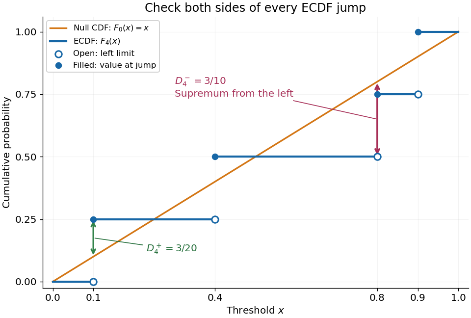
The finite formula follows from the behavior between jumps: the empirical distribution function $F_n$ is constant and the cumulative distribution function $F_0$ is monotone, so the largest directional gaps occur at the two interval ends, possibly as one-sided limits. The two tails introduce no larger gap. Checking every jump side therefore gives the exact supremum.

A common normalized Kolmogorov-Smirnov statistic is $\sqrt{n}{D}_n$, which equals $3/5$ in this example. Its large-sample reference law comes from the Kolmogorov-Smirnov theorem. The unscaled $D_n$ remains the largest difference of cumulative probabilities, not a p-value.

There is a useful exact exception to the usual warning about fitting statistical parameters. Suppose $n\ge 2$ independent and identically distributed observations have the uniform distribution on $(0,\theta )$ with unknown $\theta >0$. Let $M={\max }_i{X}_i$ and let $J$ be the label of its almost surely unique maximizing observation. Conditional on $M=m$ and $J=j$, the surviving labelled observations $(X_i{)}_{i\ne j}$ are independent with the uniform distribution on $(0,m)$; after division by $m$ they are independent and identically distributed uniforms on $(0,1)$. These are conditional distributions defined by probability density functions, since the event $M=m$ has probability zero.

To check this, the joint probability density function of $M$ and $J=j$ is $m^{n-1}/{\theta }^n$ for $0<m<\theta$. Dividing the original joint probability density function ${\theta }^{-n}$ by this factor gives the conditional survivor probability density functionThis factorization proves the claimed conditional independence; scaling removes $m$. Keep the surviving labels in a fixed order, or apply an independent random permutation. The sorted survivors instead have the joint law of uniform order statistics and exhibit statistical dependence; sorting does not affect their empirical distribution function. Delete the maximum itself, which would otherwise become a forced value $1$, and compute the Kolmogorov-Smirnov statistic using sample size $n-1$ and jump heights $i/(n-1)$. This gives an exact conditional Kolmogorov-Smirnov test under the uniform-endpoint statistical model. It does not justify fitting an arbitrary endpoint or other statistical parameters and using the ordinary $n$-sample calibration.