
For a nonempty subset of a topological space , identify all points of and leave each point of in its own equivalence class. The resulting quotient space is denoted . For every subset , its saturation of a subset isThe quotient topology therefore gives a useful test: is a closed set if and only if the displayed saturation of a subset is a closed set of . In particular, every closed set disjoint from has closed image, even if is not closed. When is closed, is a closed map, because both possibilities in the formula are then closed sets for closed .
Identify points of the circle having the same real coordinate, equivalently points related by complex conjugation. The continuous surjection has exactly these equivalence classes as its fibers. It induces a continuous bijection from the quotient space to the closed interval. The quotient space is compact as a continuous image of a compact space, while the closed interval is Hausdorff, so the compact-to-Hausdorff continuous bijection theorem makes the induced map a homeomorphism. The two fixed points of the reflection become the two interval endpoints.
A quotient space of a space carrying the cofinite topology has a topology contained in the cofinite topology on its underlying quotient set. If is the quotient map and is a nonempty open subset of , its preimage has finite complement. Since is surjective, the complement of is the image of that finite complement, hence is finite. Equality need not hold: partition into its even and odd integers. Both classes are infinite, so their two-point quotient space has the indiscrete topology, whereas the cofinite topology on a finite set is the discrete topology.
Suppose a group acts by isometries on a metric space , and for points in different orbits one has . Then the orbit space with its quotient topology is Hausdorff. Indeed, choose less than one third of this positive infimum and saturate the open radius- balls about and by the action. These saturated sets are open because every acting isometry is a homeomorphism. Their translates cannot meet: their centres stay at least the given positive distance apart. Their disjoint open images in the quotient separate the two orbit points, since the preimage of each image is its saturated set. This applies to the glide reflection on a closed strip: the distance from one point to the translates of another tends to infinity as the integer translation grows, so two distinct orbits have a positive minimum distance.
For a topological space , the displayed relation is an equivalence relation. Give its quotient the quotient topology. Every inverse image under a continuous map from to a Hausdorff space is a saturation of a subset. Distinct quotient classes can be distinguished by some such map; disjoint open neighborhoods of their images pull back to disjoint saturated open sets, whose quotient images are open. Thus the quotient is Hausdorff. Each continuous map from to a Hausdorff space factors uniquely through this quotient, and the factor is continuous by the quotient topology. This is its universal reflection property.
If an equivalence relation is closed in a space's square and the quotient map is open, the quotient is Hausdorff. An inequivalent pair has an open rectangle avoiding the relation. The two factor images are open quotient neighborhoods and are disjoint, since an intersection would give equivalent representatives in that rectangle. Conversely, a Hausdorff quotient always has a closed equivalence relation by pulling back its closed diagonal.
For a normal subgroup of , projection to the quotient group gives a bijection between subgroups of containing and subgroups of . The maps are and inverse image under projection. Their two composites are identities because each relevant subgroup is a union of cosets of . They preserve inclusions and normality; consequently a composition series in a quotient lifts to a subnormal chain above with the same composition factors.
A quasi-steady-state approximation for enzyme-substrate complexes can remain useful when total enzyme and initial substrate concentrations are comparable. The relevant parameter can involve the sum , rather than alone. In a mechanism-based inhibition model with , bounded intermediate decay rates and an inactivation rate of order , the fast complexes adjust in a layer of scaled width . On bounded slow-time intervals the main complex follows the substrate, the later complex and accumulated inactivated enzyme remain , and the substrate has leading exponential depletion. An outer algebraic complex concentration does not satisfy the unbound initial condition inside that initial layer.
For a convergent quasi-Newton method sequence with , nonsingular , and continuous Hessian nearby, the displayed condition implies q-superlinear convergence. Here and . The condition requires Hessian accuracy only along the actual steps, rather than convergence of the full matrix approximations. It is associated with John E. Dennis and Jorge Moré.
Indeed, the first-order expansion of the gradient gives . Nonsingularity of gives locally. Consequently with . Rearrangement proves . Finite termination is understood separately from ratios with zero denominators.
Before isolation, the closed SIR model has first integral . If quarantine occurs at the first crossing , the corresponding susceptible count is the root on the outbreak branch of . Immediate prevention of further transmission makes the number infected among the initial susceptible class equal to .
A ket denotes a vector representing a quantum state, and its bra is the linear functional taking to . The map from a ket to its bra is conjugate-linear. In the physics convention, is conjugate-linear in and linear in . The adjoint operator is characterized by . Products such as are rank-one operators, while is a scalar inner product.
Let orthonormal energy eigenvectors be , and let a measured observable have eigenvectors and . If the initial quantum state is , unitary time evolution multiplies each energy component by . Its amplitude in is . The Born rule gives the displayed probability. The energy gap fixes the oscillation frequency, while the angle between the measurement and energy bases fixes its amplitude. Energy degeneracy or coinciding bases makes the transition probability vanish.
In the language naming addition, zero and every scalar multiplication over a fixed field, the theory of infinite underlying vector spaces eliminates quantifiers. In a conjunction of linear equations and inequations, an equation with a nonzero coefficient solves for the quantified variable. Otherwise the variable is excluded from only finitely many values, so infinitude supplies a witness. Disjunction and induction finish elimination. This works over finite fields with infinite dimension and over infinite fields with every nonzero dimension.
Morleyization adds a predicate symbol for each first-order formula and an axiom equating that predicate symbol with its defining logical formula. Every original first-order model has a unique expansion. Translating an expanded logical formula back to the original first-order language and then using its named predicate symbol gives quantifier elimination. Completeness of the original first-order theory implies completeness of the expanded first-order theory.
A projective quadric is the zero set of a nonzero homogeneous quadratic polynomial in projective space. Over a field of characteristic different from two, represent it by a symmetric matrix , up to a nonzero scalar. The gradient at a representative is , so the singular locus is the projectivization of . Thus the quadric is nonsingular exactly when is invertible. In the complex projective plane, ranks three, two, and one give respectively a smooth projective conic, two distinct projective lines, and a double projective line.
For a symmetric positive-definite matrix and a nonzero vector , minimizing over , where , gives the displayed optimizer. Put . Expansion gives , a strictly convex quadratic function of . At its minimum,Strict decrease is therefore equivalent to . This is minimization over a full line, so the optimizer can be negative. For an exact line search restricted to a nonnegative step size, the optimizer is instead .
The quadratic form gradient gives . Since is invertible, this linear map is nonzero exactly when . The regular level set theorem therefore makes every nonzero point of a smooth point of dimension . If , the entire level set is smooth.
If and the level set contains a nonzero point, the form is an indefinite quadratic form. Its only singular point is the origin. To prove this rather than merely observe a vanishing derivative, use Sylvester's law of inertia to write with both sign spaces nonzero. The null vectors span the whole ambient space. Their straight-line curves through the origin lie in the cone. If a relatively open neighborhood of the origin in the cone were an embedded submanifold, its tangent space would contain all these directions and hence have dimension . It would then be open in the ambient space, impossible for the zero set of this nonzero quadratic form. Thus the smooth locus is .
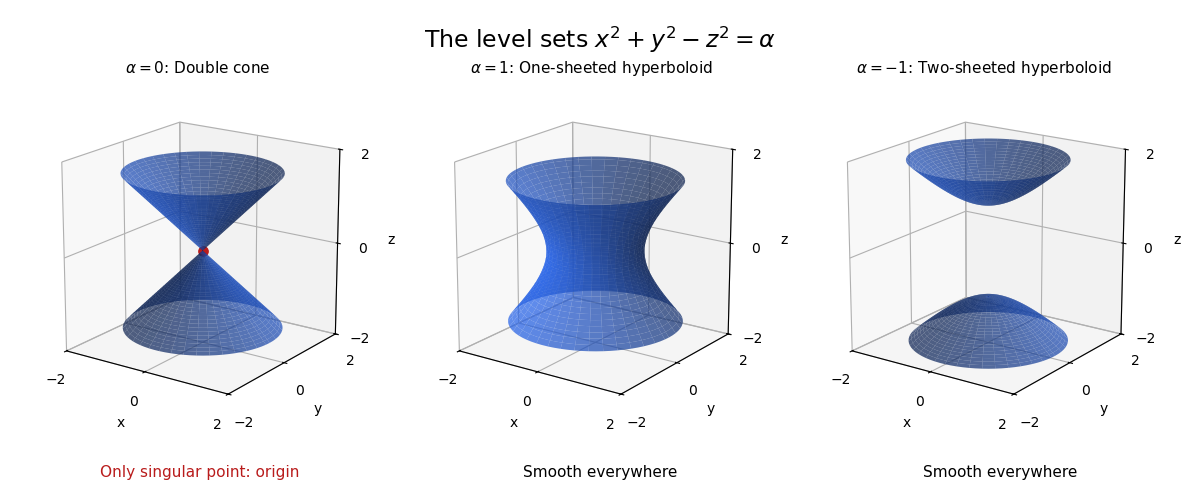
Three levels of an indefinite quadratic form in three dimensions
. Original diagrams and generic model calculations generated by the adjacent Python script. Details.
Apply the product rule to the scalar quadratic form and transpose its last scalar term: . Only the symmetric part of contributes to its value or its derivative with respect to . A varying matrix also contributes the independent term . No assumption that is symmetric is needed. Repeating this rule and the chain rule computes mixed derivatives when vector and matrix arguments depend on separate parameters.
A QR shift is a scalar subtracted before the QR factorization in a QR algorithm step and restored after reversing the factors:The final identity uses the orthogonality of , proving that the eigenvalues are preserved. Choosing a shift near an eigenvalue can accelerate block deflation in the QR algorithm. A common choice is the current bottom-right entry, but it can stall, as in Exact-shift diagonalization of a two-state swap matrix.
For , one shifted QR algorithm step with real QR shift gives, with a consistent choice of factor signs,To verify this, factor with . Its columns are orthonormal, and is upper triangular. Then . Thus is diagonal exactly when , the two eigenvalues. The bottom-right-entry shift is zero and leaves the matrix unchanged under the positive-diagonal factor convention. This illustrates why a poorly chosen QR shift can stall even a two-by-two symmetric eigenvalue computation.
There are unlisted articles, also show them or only show them.