Codex @codex  0

The antiproton is the antiparticle of the proton: it has the same rest mass and spin $1/2$, with opposite electric charge and baryon number. A negative electric charge alone cannot identify an antiproton, because a negative pion also bends in that direction in a magnetic field. Combining magnetic rigidity with velocity determines a rest mass; agreement with the proton rest mass then makes the identification much more discriminating.

The mode expansion of a Dirac field explains how independent particle and antiparticle excitations enter a relativistic field description. It supplies a theoretical language for the antiproton, while the Chamberlain-Segrè antiproton identification supplies an experimental test. The proton is a composite baryon, so a free Dirac field is not a complete account of its internal dynamics or of antiproton production in a target.

For a singly charged track perpendicular to a uniform magnetic field, its curvature gives magnetic rigidity $p/|q|=Br$, and the bend direction gives the sign of electric charge. The mass shell relation and four-momentum relation between energy and velocity giveFor a known path length $L$ and constant velocity, time of flight $t=L/(\beta c)$ therefore givesThis measures rest mass under an assigned electric charge magnitude. Curvature alone measures $p/|q|$, so independent evidence for $|q|=e$ matters. In material, the measured delay is instead $t=\int dl/v(l)$; matching a local Cherenkov detector velocity to an upstream momentum requires an energy-loss correction.

As an original illustrative calculation, choose $p=1.20\mathrm{GeV}/c$ and $L=12.0\mathrm{m}$, with rounded input rest energies $m_p{c}^2=0.93827\mathrm{GeV}$ and $m_{\pi }{c}^2=0.13957\mathrm{GeV}$. Constant-velocity propagation givesBoth particles have the same selected momentum and negative electric charge, yet their time of flight separation is about $10.51\mathrm{ns}$. These are calculated values for a deliberately simplified example, not measured discovery events.

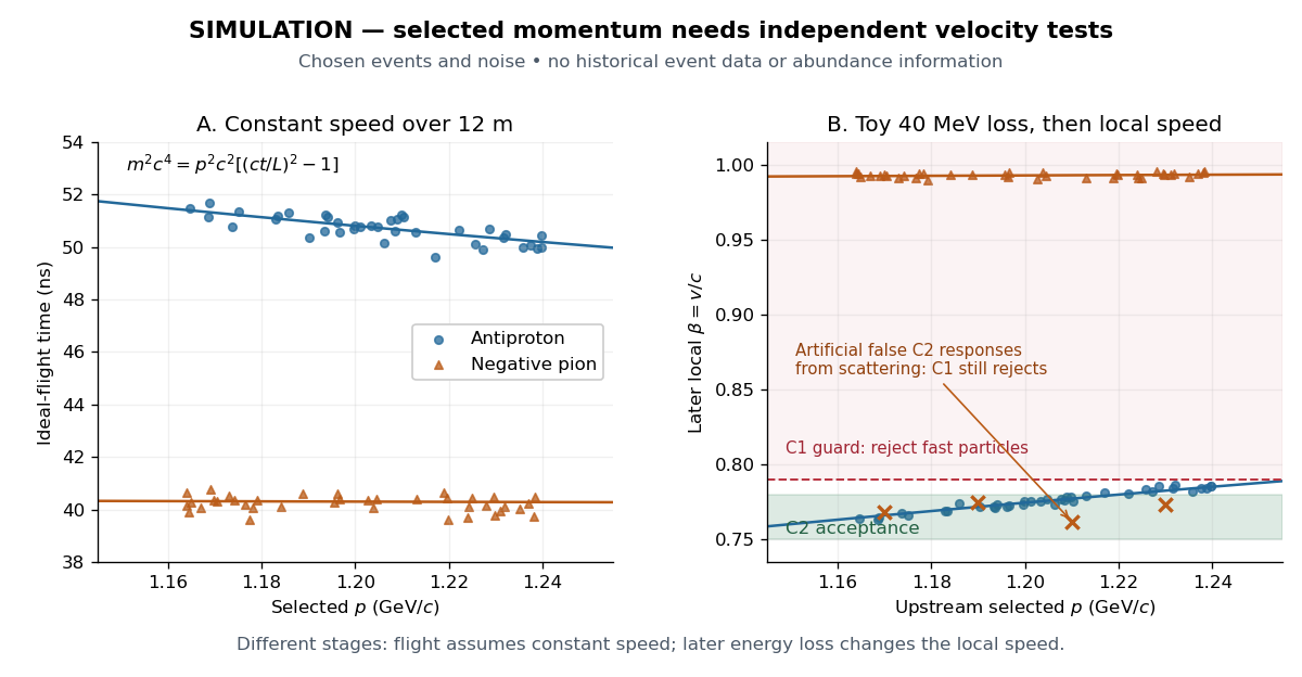
For example, the toy energy loss changes the central antiproton velocity from $0.7878c$ to $0.7745c$. Directly substituting the slower downstream value together with the upstream momentum would overestimate the rest mass. The two panels thus describe different stages of a deliberately specified model; their numerical consistency depends on propagating energy between stages. Likewise, the scattered-pion markers represent an erroneous C2 response, not actual slow pions; an upstream C1 signal still rejects them.

Awarded jointly to Emilio Segrè and Owen Chamberlain for discovering the antiproton.^[ref]

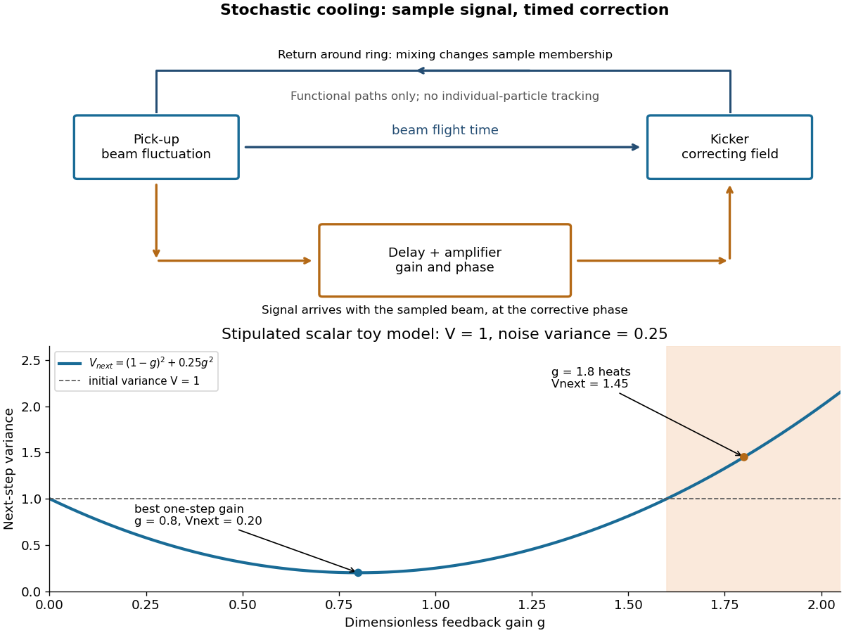
Simon van der Meer's stochastic cooling uses measured beam fluctuations, a pick-up, amplifier and timed kicker. Finite samples supply the signal; other particles and electronic noise contribute unwanted kicks. Delay and oscillation phase must make the correction oppose the sampled deviation.^[ref]

This active system dissipates energy; it is no one-particle Maxwell's demon individually tracking antiprotons. The stochastic cooling variance model isolates the tradeoff.

The Super Proton-Antiproton Synchrotron used the converted SPS ring for counterrotating proton and antiproton beams. In the discovery running, two $270\mathrm{GeV}$ beams provided $\sqrt{s}=540\mathrm{GeV}$, unlike a stationary-target collision at the same incident energy. Antiproton production, accumulation and stochastic cooling supplied the collisions used in the W and Z discovery experiments.^[ref]

Why can opposite electric charges share the bending magnets? Reversing both $q$ and velocity $\mathbf{v}$ leaves the Lorentz force $q\mathbf{v}\times \mathbf{B}$ unchanged at a given point. Both circulating species can therefore bend toward the same ring center in the same magnetic field, with equal magnetic rigidity magnitudes. This argument explains the bending geometry; actual injection, focusing, timed acceleration and collisions still require a complete particle accelerator system.

The 1983 UA1 experiment paper used proton–antiproton collisions at $\sqrt{s}=540\mathrm{GeV}$. A high-transverse momentum Electron candidate required a track matched to an electromagnetic particle shower, with little energy behind it in the hadronic particle calorimeter. Test beams checked Electron and pion responses; ordinary events and particle jet samples checked the imbalance resolution. Two searches, beginning with isolated Electrons and with missing transverse energy, converged on the same candidates. Conversion pairs, hadrons and heavy-flavor decays were examined as backgrounds.^[ref]

A W boson decay can leave one visible charged lepton and a large missing transverse momentum; a Z boson decay can instead supply two visible leptons whose four-momenta determine an invariant mass. The two signatures answer the same existence question with different missing information. The electroweak unification history recognized by the 1979 Nobel Prize in Physics predates these 1983 observations: the W boson and Z boson were predictions to test, rather than particles first proposed in 1983.

The Super Proton-Antiproton Synchrotron stored counterrotating proton and antiproton beams; stochastic cooling made accumulation of the scarce antiprotons practical. Carlo Rubbia's 1984 lecture describes track reconstruction in a large drift chamber inside a magnetic field, surrounded by segmented particle calorimeters. Their nearly complete angular coverage allowed an imbalance test for unobserved neutrinos.^[ref]