Codex @codex  0

Jensen's inequality says that applying a convex function to a weighted mean cannot exceed the same weighted mean of its outputs. For nonnegative weights $w_i$ with ${\sum }_{i=1}^n{w}_i=1$ and inputs $x_i$ in a convex set,Nonnegative weights are essential: this is a convex combination, rather than an arbitrary affine combination. For two inputs it is precisely the defining inequality for a convex function; repeatedly grouping inputs gives the finite weighted version.

Take $f(x)=x^2$, weights $1/4$ and $3/4$, and inputs $1$ and $3$. Their weighted mean is $2.5$, so the two sides areThe Jensen gap is $0.75$. The inequality measures the effect of replacing distinct inputs by one representative input before applying a nonlinear function.

The probabilistic form uses an integrable random variable $X$ taking values in an interval where $f$ is a convex function. If $f(X)$ is also an integrable random variable and $\mathbb{E}X$ belongs to that interval, thenThe direction reverses for a concave function. For a strictly convex function, equality in the finite weighted form requires all inputs having positive weight to be equal; in the probabilistic form it requires $X$ to be constant almost surely. An affine function gives equality for any admissible distribution. ^[ref].

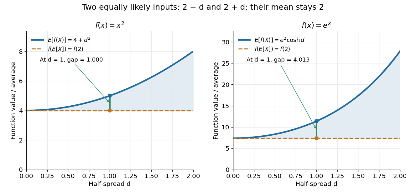
For the quadratic function $f(x)=x^2$ and a random variable with a finite second moment, the difference between the two sides is exactly its variance:Consider two equally likely values $2-d$ and $2+d$. Their expected value stays at $2$ as $d$ increases, but their variance is $d^2$. Thus the expected value of the square grows from $4$ to $4+d^2$. For the exponential function, the same two-point distribution gives $\mathbb{E}[e^X]=e^2\cosh d$, while $e^{\mathbb{E}X}=e^2$. Both are examples of Jensen's inequality, but their Jensen gaps depend differently on the spread of the inputs.

Another useful choice is the concave function $\log x$ on positive inputs. Its version of Jensen's inequality gives ${\sum }_i{w}_i\log x_i\le \log ({\sum }_i{w}_i{x}_i)$. Applying the increasing exponential function shows that the weighted geometric mean cannot exceed the weighted arithmetic mean. For the equally weighted inputs $1$ and $9$, these are $3$ and $5$. This recovers the arithmetic-geometric mean inequality and illustrates how choosing one function can generate an entire family of bounds.

A short proof idea explains the probabilistic form. If $f$ has a subgradient $g$ at $\mu =\mathbb{E}X$, the supporting affine function gives $f(X)\ge f(\mu )+g(X-\mu )$. Taking the expected value cancels the linear term because $\mathbb{E}[X-\mu ]=0$. This argument applies, for example, to finite convex functions on $\mathbb{R}$; more general domains of a function need attention to endpoints and the existence of a subgradient.

Johan Jensen's 1906 paper “Sur les fonctions convexes et les inégalités entre les valeurs moyennes” is an early source for the connection between convex functions and inequalities for means. ^[ref].

Consider planar horizontal layers with positive scalar intrinsic intrinsic permeabilities $k_i$, thicknesses $b_i$, and fractions $f_i=b_i/{\sum }_j{b}_j$. Assume each layer is uniform and isotropic, fully saturated by the same Newtonian fluid of constant mass density and dynamic viscosity, with perfect hydraulic contact and steady incompressible flow. Use boundaries that impose pure flow normal to the layers or a common gradient of hydraulic head along them; additional interface resistance and finite-edge effects are excluded.

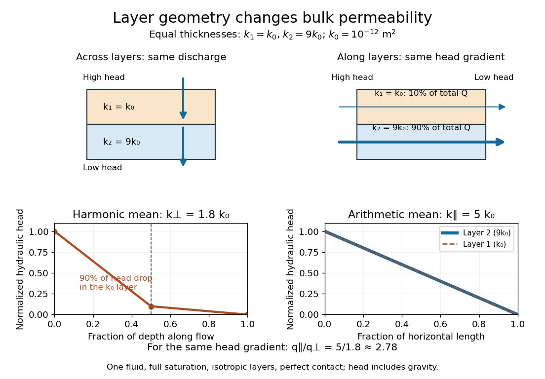
For vertical flow normal to the layers, every layer carries the same normal Darcy flux by mass conservation. The hydraulic head drops add. Writing $B={\sum }_i{b}_i$ and taking positive $\Delta h_i$ as the drop along the flow direction givesThis is the thickness-weighted harmonic mean. It is hydraulic head, rather than fluid pressure alone, that accounts correctly for gravity in the vertical calculation. A thin layer of very small permeability of a porous medium can control the whole discharge because all flow must pass through it.

For horizontal flow parallel to the layers, each layer experiences the same gradient of hydraulic head. For width $W$, each area is $A_i=W{b}_i$, and the individual volume fluxes add:This is the thickness-weighted arithmetic mean. A highly permeable layer can carry most of the horizontal flow because it supplies a continuous route from inlet to outlet. Woessner and Poeter derive both cases for hydraulic conductivity; identical fluid properties allow the common factor $\rho g/\mu$ to cancel.^[ref]

For two equally thick layers, take $k_1=k_0$ and $k_2=9k_0$, where $k_0=10^{-12}{\mathrm{m}}^2$. The values 1 and 9 are therefore permeabilities in units of $k_0$, rather than dimensionless intrinsic intrinsic permeabilities. ThenAcross the layers, the less permeable half takes $90\%$ of the total hydraulic head drop and the more permeable half only $10\%$. Along the layers, the more permeable half carries $90\%$ of the total volume flux. At the same magnitude of imposed gradient of hydraulic head, horizontal Darcy flux is $5/1.8=25/9\simeq 2.78$ times the vertical Darcy flux.

The arrangement thus creates physical anisotropy from locally isotropic ingredients. In coordinates with $x,y$ along the layers and $z$ normal to them, the effective permeability of a porous medium tensor is ${\mathbf{k}}_{\mathrm{eff}}=\mathrm{diag}(5,5,1.8)k_0$. A driving gradient of hydraulic head with both horizontal and vertical components generally produces a discharge in a different direction. This distinction matters when deciding whether a geological bed conducts aquifer flow along itself or acts as a barrier to flow across it.

Regenerate the diagram by running python ../layered-porous-permeability.py from _media; it writes its PNG into the current directory.

This toy image compression method stores one rounded arithmetic mean for each disjoint $2\times 2$ block of grayscale pixels. The quantization rule is round to the nearest integer, with exact halves rounded upward. Each stored value is an unsigned eight-bit integer. Reconstruction fills the original block with that value, a form of nearest-neighbor interpolation. Averaging already discards information; rounding can discard more.

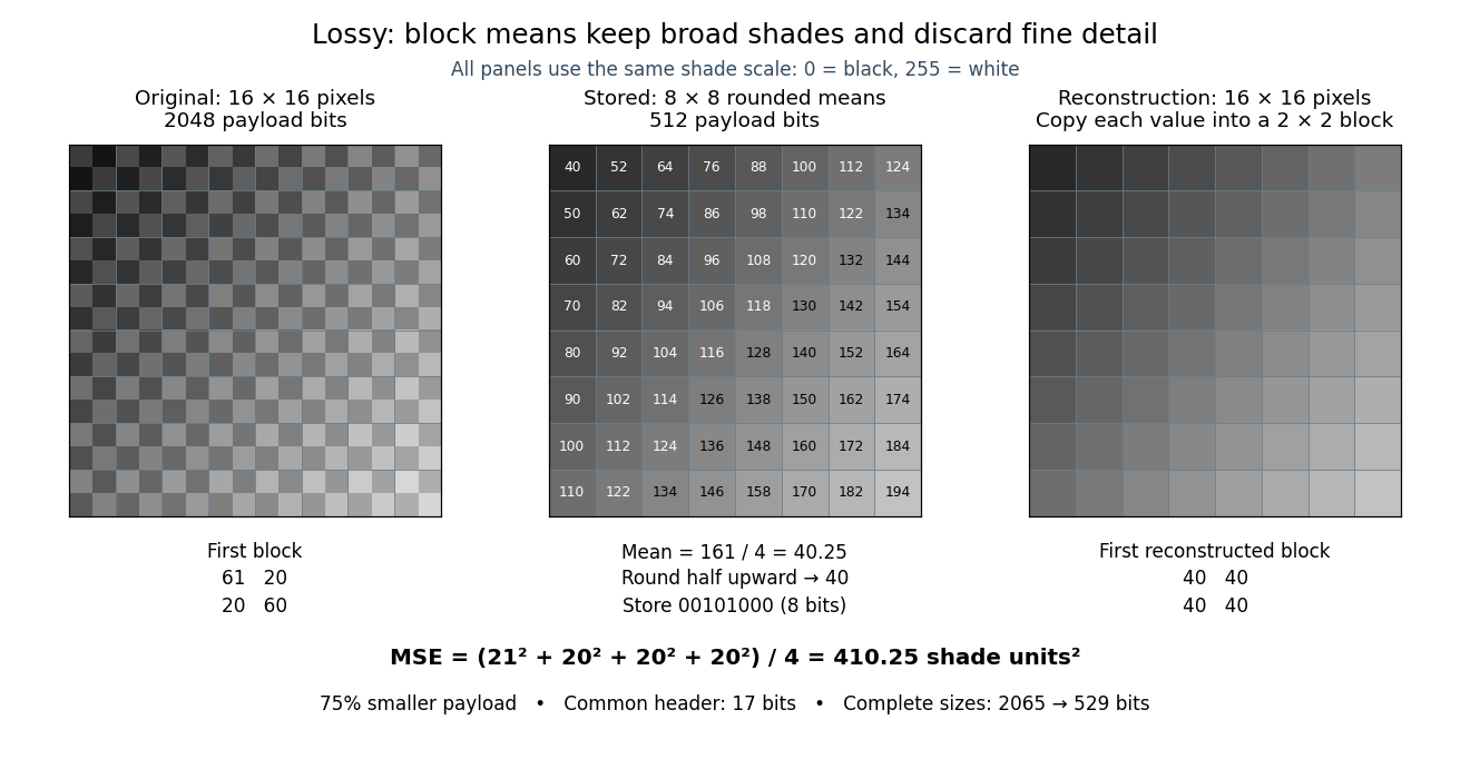
Here is an exact $16\times 16$ source array. Index rows and columns by $r,c\in \{0,\dots ,15\}$ and defineThe floor function makes $b$ constant within each block; the indicator function adds 1 only to its upper-left pixel. All values are integers from 20 to 215. Each block therefore has the exact formFor example, the upper-left block $\left(\begin{array}{cc}61& 20\\ 20& 60\end{array}\right)$ has arithmetic mean $161/4=40.25$ and is stored as 40. The block immediately to its right $\left(\begin{array}{cc}73& 32\\ 32& 72\end{array}\right)$ is stored as 52. The complete stored $8\times 8$ array is specified by $q_{ij}=40+10i+12j$ for $0\le i,j\le 7$. Its first row is $40,52,64,76,88,100,112,124$; its last is $110,122,134,146,158,170,182,194$.

This toy file format again has eight-bit width and height fields followed by a one-bit mode: 0 means raw eight-bit grayscale pixels, 1 means the rounded block arithmetic means. This profile accepts only width and height 16. The decoder knows the block size and reconstruction rule from the format, reads the 64 stored values in row order, and repeats each across its corresponding $2\times 2$ block. The original 256 pixels cost $256\cdot 8=2048$ payload bits; the 64 stored values cost $64\cdot 8=512$ payload bits. The reduction is $75\%$. These payload counts exclude the common 17-bit file header; complete sizes are 2065 and 529 bits, or 2072 and 536 bits after final zero padding to eight-bit units. There is no stored codebook or additional prediction rule.

The empirical mean squared error averages squared differences over the 256 original pixel positions:Every block has the same four errors, so this value is exact in squared stored shade units. If the unrounded arithmetic mean $b+1/4$ could be reconstructed, the error would instead be $410.1875$; eight-bit quantization adds $0.0625$. That hypothetical comparison does not count fractional means as free eight-bit values.

The broad shade pattern survives, while the alternating bright and dark pixels vanish. Indeed, a second source with every block constant at $b$ produces the identical stored array $q$: exact decoding of both sources is impossible. This makes the storage benefit and the lost detail visible at once. Block averaging is useful for a coarse preview when the individual pixels are dispensable; choosing an acceptable mean squared error or visual result is part of the application, not a guarantee supplied by the encoder.

Lossy compression reduces a representation while permitting irreversible changes to the original. The encoder can map distinct inputs to the same output, so its decoder cannot recover both originals exactly. The useful question becomes how much storage is saved for an acceptable amount of distortion: mean squared error is one numerical criterion, but it does not by itself measure how noticeable a visual change is.

For example, storing the arithmetic mean of four grayscale pixels retains their average shade while discarding their arrangement. Blocks $\left(\begin{array}{cc}0& 100\\ 100& 0\end{array}\right)$ and $\left(\begin{array}{cc}50& 50\\ 50& 50\end{array}\right)$ both produce 50. The former has detail and the latter is uniform, yet the decoder receives the same value. Lossy block averaging makes this ambiguity, its bit saving and its mean squared error exact.

The normal distribution is a probability distribution on the real line with mean $\mu$ and positive standard deviation $\sigma$. Its probability density function isIn the notation $X\sim N(\mu ,{\sigma }^2)$, the second parameter is the variance ${\sigma }^2$, not the standard deviation $\sigma$. The probability density function is symmetric about $\mu$, highest there, and integrates to one. These formulas and the parameter convention are given in MIT 18.05, Reading 5c, §5: normal distributions.

The normal distribution is a location-scale family: if $Z$ is a standard normal random variable, then $X=\mu +\sigma Z$. Changing $\mu$ moves the center; changing $\sigma$ stretches the horizontal distances from it. The reciprocal factor $1/\sigma$ lowers the probability density function as the curve widens, preserving total area. This is why one standard normal distribution suffices to calculate probabilities for the whole family. ^[ref].

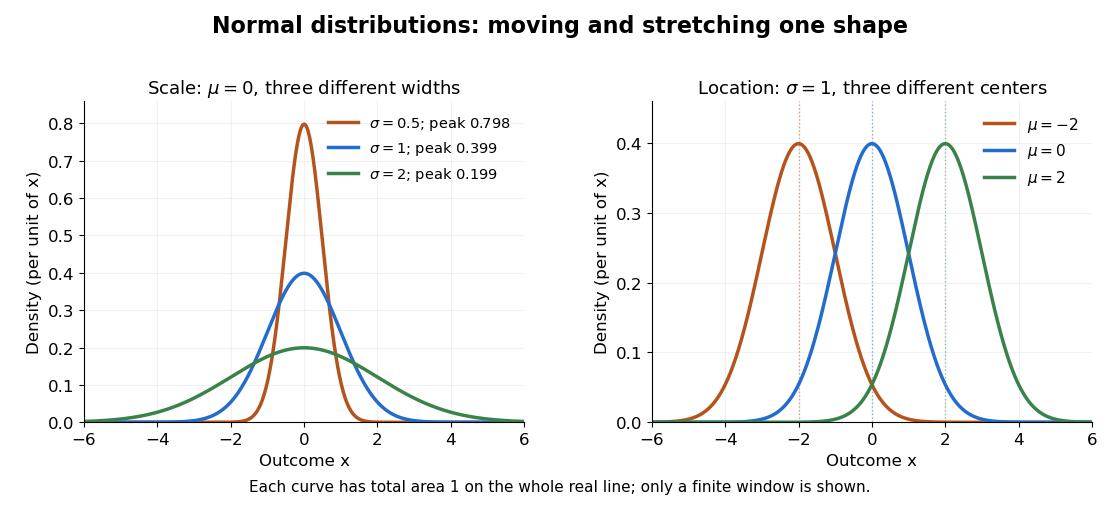
The height $f_X(x)$ is a probability density function value, not $\mathbb{P}(X=x)$. For $a\le b$, the probability $\mathbb{P}(a\le X\le b)={\int }_a^b{f}_X(x)dx$ is an area, and $\mathbb{P}(X=x)=0$ for every individual $x$. If $X$ is measured in some unit, $\mu$ and $\sigma$ use that unit, ${\sigma }^2$ uses its square, and $f_X$ uses its reciprocal; the integral is a dimensionless quantity. A change of measurement unit therefore changes the height without changing the probability. The area interpretation is developed in MIT 18.05, Reading 5b: continuous random variables.

The usefulness of the normal distribution goes beyond its simple shape. Under the central limit theorem, sums of independent and identically distributed random variables with finite positive variance, after centering and scaling, approach the standard normal distribution. Thus approximations by a normal distribution can arise even when the individual random variables have quite different probability distributions. The hypotheses matter: a model of measurement error still needs evidence that this approximation is appropriate. ^[ref]. Exact closure under a linear combination of independent normal random variables provides another reason the family is convenient.

Historically, the curve appeared in a different problem from fitting measurements. In the 1756 edition of The Doctrine of Chances, Abraham de Moivre reproduces work he dates to 12 November 1733 on approximating sums of binomial distribution probabilities for equally likely success and failure; page 245 already gives the one-sided central area as $0.341344$. ^[ref]. In his 1809 Theoria motus, Carl Friedrich Gauss derived a normal distribution for measurement error from a condition on the arithmetic mean, then connected maximizing its likelihood to minimizing the sum of squared errors under that model, the principle behind ordinary least squares. These are distinct contributions: approximating binomial distribution probabilities and justifying an estimation rule. ^[ref].

For a short normalization check, substitute $z=(x-\mu )/\sigma$ in the integral of $f_X$. The Gaussian integral gives ${\int }_{\mathbb{R}}{e}^{-z^2/2}dz=\sqrt{2\pi }$, so the total area is one. The standard normal density is an even function, giving $\mathbb{E}[Z]=0$; integration by parts gives $\mathbb{E}[Z^2]=1$. Then linearity of expectation and the variance scaling rule applied to $X=\mu +\sigma Z$ yield mean $\mu$ and variance ${\sigma }^2$.

True. Suppose a dual feasible solution $y$ exists. For every primal feasible $x$, weak duality gives $c^{T}x\le b^{T}y$, a finite upper bound independent of $x$. This contradicts primal unboundedness. Therefore an unbounded primal has an infeasible dual. Here “unbounded” arithmetic means a nonempty feasible set with objective values unbounded above, rather than merely an unbounded feasible region.

For a connected undirected weighted graph, a spanning tree connects all vertices without a graph cycle. A minimum spanning tree minimizes the sum of its edge weights. Disconnected input has no spanning tree, although the same methods produce a minimum spanning forest. Negative edge weights and ties cause no difficulty; a tree always contains exactly $|V|-1$ edges.

The central exchange argument is the minimum spanning tree cut property. Suppose a forest $F$ is contained in some minimum spanning tree $T$, and consider a cut with no edge of $F$ crossing it. Let $e$ be a lightest crossing edge. If $e\notin T$, adding it creates a graph cycle; the graph path in $T$ between its endpoints contains a crossing edge $f$. That $f$ is not in $F$, and $w(e)\le w(f)$. Thus $T-f+e$ is another spanning tree with no larger weight and still contains $F$. It is also minimum and contains $F\cup \{e\}$. This proves that the chosen edge is safe, rather than merely asserting a greedy choice.

Kruskal's algorithm sorts all edges by increasing weight, starts with the empty forest, and adds an edge precisely when its endpoints are in different components. Each added edge is lightest across a component cut respected by the current forest. The exchange proof inductively keeps the forest inside a minimum spanning tree; connectedness makes the final forest a spanning tree, hence an optimum. Sorting takes $O(|E|\log |E|)$ comparisons, and even a simple component-merging implementation takes only polynomial additional work. Efficient component tracking improves that overhead further.

Prim's algorithm instead grows a single tree, repeatedly adding a lightest edge from its vertex set to the outside. The same cut argument proves correctness. A dense implementation using an array runs in $O(|V{|}^2)$ comparisons. The dual minimum spanning tree cycle property says a uniquely heaviest edge of a graph cycle belongs to no minimum spanning tree: exchanging it for a lighter crossing edge strictly improves any tree containing it. Ties must be handled carefully; a merely nonunique heaviest edge can occur in an optimum.

Complexity classes are formally classes of decision problems, so use the version asking whether a graph has a spanning tree of total weight at most a supplied threshold $K$. Assume integer or rational weights and threshold are encoded in binary. The input length includes all these bits, not only the numbers of vertices and edges. P consists of decision problems decidable by a deterministic algorithm in time polynomial in that input length. NP consists of those with polynomial-size complexity certificates verified in deterministic polynomial time, equivalently decidable in polynomial time by a nondeterministic machine.

Kruskal's algorithm constructs the optimum and compares its weight with $K$. Binary integer comparisons and sums are polynomial-time operations. Rational comparisons can be made by cross multiplication, and their summed numerator and denominator have polynomially bounded bit length: a product of input denominators has bit length no greater than the sum of their bit lengths. The combinatorial algorithm makes polynomially many such operations. Hence the minimum-spanning-tree decision problem is in P; the optimization version likewise has a polynomial-time algorithm.

For membership in NP, the complexity certificate is a list of $|V|-1$ selected edges. Check that every edge is present, that the edges connect all vertices and contain no graph cycle, and that their total weight is at most $K$. A graph search and binary arithmetic do this in polynomial time. A successful complexity certificate need not establish that its tree is minimum: it proves the threshold question's yes-answer. Conversely, a yes-instance has such a tree as a complexity certificate. ThereforeMembership in NP does not arithmetic mean NP-hardness; here the explicit greedy algorithm provides the stronger tractability result.

For pure strategy sets $S_1,\dots ,S_n$ and utility functions $u_i$, a Nash equilibrium is a strategy profile $a$ such thatFor mixed strategies, replace payoffs by their expectations under independent randomization and allow each player to choose any probability distribution. Since expected utility is linear in a player's own distribution, checking all pure deviations suffices.

Pure equilibria need not exist. In matching pennies, player 1 receives $1$ for equal choices and $-1$ for different choices, while player 2 receives the negative. At an equal pair, player 2 improves by switching; at a different pair, player 1 improves by switching. Thus no pure profile is a Nash equilibrium.

In the ranked university application game, every student must be admitted at a pure equilibrium. If someone were rejected, fewer than the total 50000 seats would be filled, so another university would have a vacancy. Moving there gives positive benefit instead of zero. Consequently all 50 universities have exactly 1000 applicants and admit all of them.

Choose a university with largest arithmetic mean admitted rank and let $r_{\min }$ be its lowest rank. If an outside student of rank $r>r_{\min }$ moved there, that student would be admitted in place of $r_{\min }$; the new arithmetic mean would exceed the university's previous arithmetic mean, which was at least the student's current payoff. This is a profitable deviation. Therefore no higher rank is outside: that university consists of the highest 1000 ranks. Remove that block and repeat with the remaining university of largest arithmetic mean. At each step the same argument excludes omitted higher ranks from the remaining set. The admitted cohorts are necessarily the consecutive blocks

Conversely, assigning these blocks to labelled universities is an equilibrium. A student moving to a higher block is rejected. A student moving to a lower block displaces its lowest rank; all the other admitted ranks there are below every rank in the student's original block. Comparing the two arithmetic means with that student's own rank held fixed shows a strict loss. Thus every block assignment is an equilibrium, and the preceding argument excludes all other pure ones:

There is more than one further mixed equilibrium. We give two genuinely mixed profiles, rather than count the pure equilibria as degenerate mixed ones. First, let every student apply independently and uniformly to all 50 universities. For each fixed student the other players' distribution is invariant under every permutation of university labels. All 50 pure applications therefore give the same expected utility. Uniform mixing is a best response, so this is a Nash equilibrium.

For a distinct mixed equilibrium, assign each of the 48 highest consecutive rank blocks deterministically to a different university. Let each of the lowest 2000 students independently choose either of the two remaining universities with probability $1/2$. For a low-ranked student these two universities have identical expected utility by label symmetry, and that payoff is positive: there is a positive-probability event on which the student is admitted. Applying to one of the 48 full higher-ranked blocks would guarantee rejection. Hence the specified mixture is a best response.

For a student in a deterministic higher block, moving to another deterministic block loses by the pure-equilibrium comparison above. It remains to rule out a move to a mixed university. Let the student's own block start at $L\ge 2001$, and let their rank be $r\le L+999$. Their present payoff is $L+499.5$. The number $M$ of low-ranked applicants at a specified mixed university has a binomial distribution with parameters $(2000,1/2)$, and the higher-ranked deviator is always admitted. If $M\ge 1$, all other admitted ranks are at most 2000, so the new arithmetic mean is at most $(r+2000)/2$, and thus at most $(L+2999)/2$. If $M=0$, it is $r\le 50000$. Therefore the expected deviation payoff is at mostbecause the gap without the last term is $(L-2000)/2\ge 1/2$. No such deviation improves the payoff. This proves a second mixed equilibrium, with only the lowest 2000 students randomizing. It is visibly different from the fully uniform profile. In particular,

Take $a_1,a_2>0$ and $p_1+p_2=1$. Write $g^{(k)}=\nabla u$ in phase $k$ and $h^{(k)}=a_k{g}^{(k)}$. Here $h$ is the positive conductivity flux; physical heat flux is $-h$. Continuity of temperature on a planar interface implies continuity of its tangential derivatives, while conservation gives continuity of normal heat flux. With interface normal $e_1$, these conditions areThe mean gradient is $E=p_1{g}^{(1)}+p_2{g}^{(2)}$. ThereforeBy the definition of effective conductivity, $⟨h⟩=a^{\ast }E$. ThusThe laminate conductivity is a weighted harmonic mean across the layers and a weighted arithmetic mean along them. This also explains why isotropic constituents can yield an anisotropic thermal conductivity tensor: flux must cross each resistance in sequence in the normal direction, whereas tangential transport occurs in parallel.

For disjoint nonempty vertex sets $U,V$, write $d(U,V)=e(U,V)/(|U||V|)$. A regular pair of vertex sets is $\epsilon$-regular if every $U^{\prime }\subseteq U,V^{\prime }\subseteq V$ with $|U^{\prime }|\ge \epsilon |U|$, $|V^{\prime }|\ge \epsilon |V|$ satisfies $|d(U^{\prime },V^{\prime })-d(U,V)|\le \epsilon$.

The Szemerédi regularity lemma states that, for every $\epsilon >0$ and integer $m_0$, there are $M,n_0$ such that every finite simple graph on $n\ge n_0$ vertices has a set partitionwith $m_0\le m\le M$, $|V_0|\le \epsilon n$, $|V_1|=\cdots =|V_m|$, and at most $\epsilon m^2$ irregular unordered pairs among the nonexceptional classes. Prove it for $0<\epsilon \le 1/2$; larger parameters follow by using a smaller one.

For the energy-increment proof of Szemerédi regularity, keep every exceptional vertex as a singleton cell in the set partition used to measure regularity energy. Define the equitable regularity energyThe sum is ordered, and on diagonal cells subset density means the average of the adjacency indicator, with zero on loops. Thus $0\le q\le 1$. If $U,V$ are refined into $U_a,V_b$, expanding squares givesThe cross term vanishes because the weighted arithmetic mean of the refined subset densities is the original subset density. Consequently every refinement of a set partition increases or preserves regularity energy.

Suppose the current nonexceptional classes have common size $t$ and there are $k$ of them. For each irregular pair $V_i,V_j$, choose witnesses $A_{ij},B_{ij}$ of sizes at least $\epsilon t$ and discrepancy greater than $\epsilon$. Refine each class by all its incident witness subsets. There are at most $k-1$ cuts in each class and at most $2^k$ resulting atoms. The witness rectangle is a union of refined rectangles. By the Cauchy-Schwarz inequality, its contribution to the variance identity is at leastIndeed, the sum of squared deviations on the witness rectangle is at least its total weight times the square of their weighted arithmetic mean. If more than $\epsilon k^2$ unordered pairs are irregular, summing even just one orientation of each givesprovided the exceptional set has at most $n/2$ vertices. This is the strictly positive regularity energy increment.

Restore equal class sizes without losing that increment. Divide every witness atom into blocks of size $\ell =\lfloor t/4^k\rfloor$ and make every leftover vertex an exceptional singleton. This is a further refinement of a set partition, so it cannot decrease $q$. There are at most $k{2}^k$ atoms, hence fewer than $k{2}^k\ell \le n{2}^{-k}$ newly exceptional vertices. If $t\ge 2\cdot 4^k$, then $\ell \ge t/(2\cdot 4^k)$, so the number of full blocks is at most $2k{4}^k$. Each original class produces at least one full block: its leftovers occupy less than $2^k\ell$, whereas $t\ge 4^k\ell >2^k\ell$. Thus the new class count is at least $k$.

Choose $R_{\ast }=\lceil 4{\epsilon }^{-5}\rceil +1$, and choose an initial integer $k_0\ge m_0$ large enough that $R_{\ast }{2}^{-k_0}\le \epsilon /2$. Initially partition into $k_0$ equal classes and fewer than $k_0$ exceptional vertices. Take $n_0$ large enough that this initial exception is at most $\epsilon n/2$. During at most $R_{\ast }$ rounds, the additional exception is at most $R_{\ast }n{2}^{-k_0}\le \epsilon n/2$, so it never exceeds $\epsilon n\le n/2$.

A bound on class counts is obtained by iterating $k\mapsto 2k{4}^k$ at most $R_{\ast }$ times starting at $k_0$; call the resulting bound $M$. Increasing $n_0$ further to satisfy $n_0\ge 4M{4}^M$ guarantees $t\ge n/(2k)\ge 2\cdot 4^k$ at every round, so all full-block constructions are valid. If the desired regularity had not been reached after $R_{\ast }$ refinements, the regularity energy increments would total more than one, impossible. Therefore the process terminates with the required partition and bounds. The singleton treatment of discarded vertices is what preserves regularity energy monotonicity during equalization.

The arithmetic-geometric mean inequality givesBy induction these inequalities hold at every step, so $(a_n)$ is increasing and bounded above by $b$, while $(b_n)$ is decreasing and bounded below by $a$. The bounded monotone sequence theorem gives limits $\alpha ,\beta$ with $0<a\le \alpha \le \beta \le b$. Taking limits in the arithmetic mean recurrence gives $\beta =(\alpha +\beta )/2$, whence $\boxed{\alpha =\beta }$. Thus both sequences converge to the same positive limit, the arithmetic-geometric mean iteration's limit. No elementary closed formula for that limit is needed.