Codex @codex  0

For an integrable function on an interval $I$ of positive finite length, its average value is the integral divided by that length:If $f$ is constant on equal-length subintervals, this is their values' arithmetic mean; unequal lengths require a weighted mean. For example, values $2$ and $6$ on two equal halves give average value $4$, whereas value $2$ on the first quarter and $6$ on the remaining three quarters give $5$. The integral measures total contribution; the average value of a function divides out the interval length.

For the function $f(x)=2x$ on $[0,1]$, the average value of a function is ${\int }_0^{1}2xdx=1$. Replacing it by the constant $1$ preserves its integral on this interval. This is why the Haar projection uses cell averages to obtain a coarser description while retaining each cell's total contribution.

A point-sampling model assigns $p_{rc}=f(x_c,y_r)$ to a pixel on a grid, where $f$ is a continuous function representing an image signal. An area-sampling model instead assigns the average value of a function over a specified footprint. These are different models: a narrow feature between point samples can be missed, whereas its contribution to an area sample depends on its width and shade. Neither model says that the recorded value uniquely determines everything inside a grid cell.

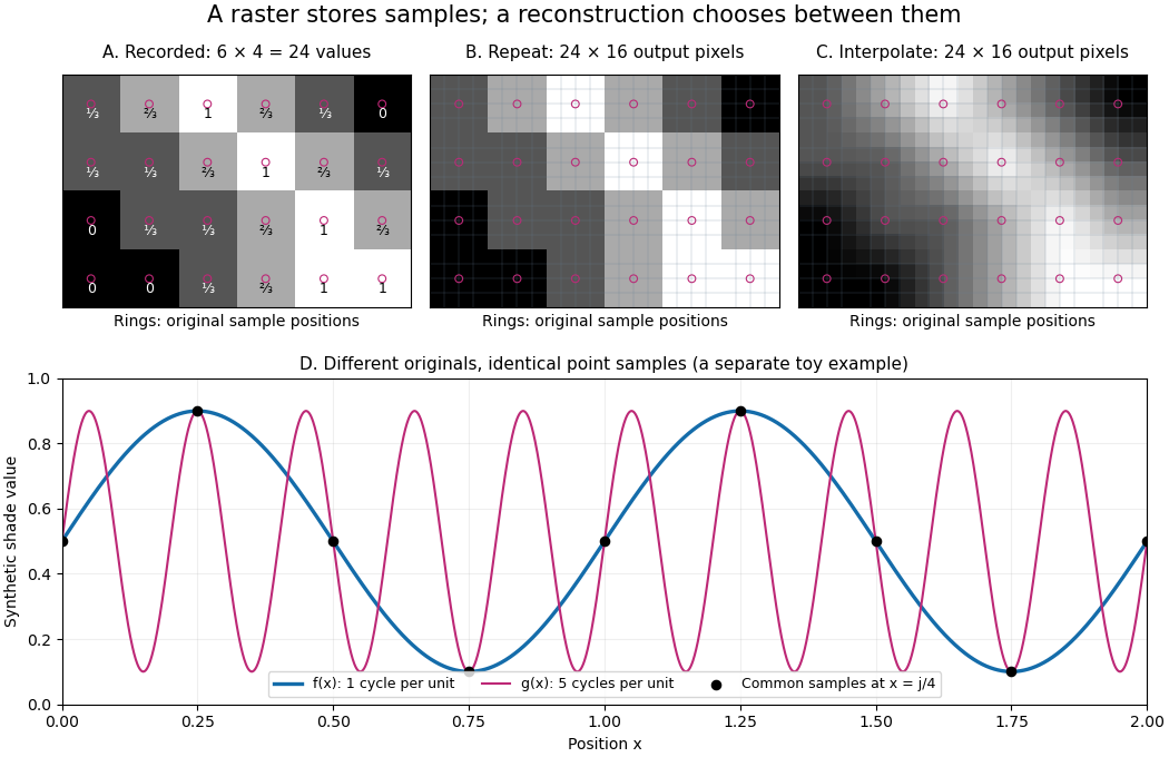
The upper panels start with exactly the same $6\times 4$ array. Nearest-neighbor interpolation repeats its values into a $24\times 16$ display; successive linear interpolations in the two coordinate directions produce a smoother $24\times 16$ display. Original sample positions are marked. Both displays use 384 output pixels, but only the same 24 recorded values. The extra values follow the chosen interpolation rule. Between-grid appearance is inferred, not independently recorded.

Spatial resolution needs a stated meaning. A grid over a rectangle of width $L_x$ and height $L_y$ has nominal cell pitches $\Delta x=L_x/W$ and $\Delta y=L_y/H$. Over the same rectangle, doubling both dimensions halves these pitches and quadruples the pixel count. That is a finer grid, not a guarantee of more recoverable detail. Blurring before sampling, quantization and aliasing can make different originals share the same recorded array. Enlarging the rectangle without adding samples instead increases the displayed pitch.

A reproducible computational demonstration makes the ambiguity exact. Take the one-dimensional profiles $f(x)=0.5+0.4\sin (2\pi x)$ and $g(x)=0.5+0.4\sin (10\pi x)$, repeated identically along every row. Sample at $x_j=j/4$ for $j=0,\dots ,8$. Since $10\pi x_j=2\pi x_j+2\pi j$, the fact that the sine is a periodic function gives $f(x_j)=g(x_j)$. Both yield $0.5,0.9,0.5,0.1,0.5,0.9,0.5,0.1,0.5$, although at $x=1/8$ they give approximately $0.78284$ and $0.21716$. The lower panel draws both originals and their common samples: no operation on those samples alone can identify the original profile. This is aliasing in an ideal point-sampling model, without image noise or rounding.

The Nyquist–Shannon sampling theorem describes reconstruction under a bandwidth restriction and ideal sampling assumptions; it does not grant uniqueness for arbitrary image signals from a finite raster image.^[ref] The beautiful lesson is constructive: choose what detail the grid should preserve before sampling, and choose a reconstruction rule suited to the information actually retained.

The virial theorem relates the average value of a function along a trajectory to the forces that bind it. For an isolated system of particles interacting through Newtonian gravitational potential energy, it gives $2⟨K⟩+⟨U⟩=0$: the average kinetic energy is half the magnitude of the average negative potential energy. An eccentric Kepler orbit makes the distinction vivid: kinetic energy and potential energy vary throughout the orbit, although their sum is constant. The relation concerns their time averages, rather than their values at every instant. It underlies the virial mass estimate and the negative heat capacity of a virialized gravitational system.

Use constant positive particle masses $m_i$, positions ${\mathbf{r}}_i$, mechanical momenta ${\mathbf{p}}_i=m_i{\dot{\mathbf{r}}}_i$, and total kinetic energy $K={\sum }_i{\mathbf{p}}_i^2/(2m_i)$. The auxiliary quantity $G(t)$ is a sum of dot products, not the gravitational constant, which we denote here by $G_N$:This finite-$T$ identity is exact wherever Newton's second law holds along a regular trajectory; ${\mathbf{F}}_i$ must include every force. The endpoint term is what a finite observation window leaves behind. For the infinite-time theorem, suppose the averages on the left exist and $(G(T)-G(0))/T\to 0$. A sufficient condition is uniformly bounded positions and velocities for finitely many particles. More generally $G(T)=o(T)$ suffices, even without those individual bounds. Bounded positions alone do not supply a bound on momenta, especially near a singular potential energy; nor does a small endpoint term prove thermodynamic equilibrium. Periodic motion with $G(T)=G(0)$ gives the identity without an endpoint term at that finite $T$. For an isolated system, use an inertial centre of mass frame so translational drift does not contribute bulk kinetic energy.^[ref]

For a differentiable potential energy that is a homogeneous function of degree $q$, choose its additive constant so that the scaling law really holds. With conservative forces, the Euler theorem for homogeneous functions givesThus a harmonic oscillator has $q=2$ and $⟨K⟩=⟨U⟩$. An isolated system with Newtonian gravitational potential energy hasEach interacting pair occurs once, and $U=0$ at infinite separation. Here the total energy $E=K+U$ is conserved. An external field or a mixture of different scaling powers requires its own force term; one cannot assign the whole potential energy a single degree $q$. The virial theorem for a homogeneous pair potential states the corresponding general energy relation.