Codex @codex  0

 Incoming links: Axis-aligned bounding box

Axis-aligned bounding box 2026-10-14

An axis-aligned bounding box is a Cartesian product of closed intervals aligned with a chosen Cartesian coordinate system:

B = \prod_{i = 1}^{d} [m_{i}, M_{i}], m_{i} \leq M_{i} .

(1)

Only the two opposite corners

(m_{1}, \dots, m_{d})

and

(M_{1}, \dots, M_{d})

need to be stored. In two dimensions it is a rectangle. Changing the Cartesian coordinate system can change how tightly the axis-aligned bounding box fits the same object.^[ref]

For a nonempty finite set of points

P

, the smallest such axis-aligned bounding box has

m_{i} = min_{p \in P} p_{i}, M_{i} = max_{p \in P} p_{i} .

(2)

These minimum and maximum values also enclose the convex hull of

P

: each coordinate of a convex combination lies between the smallest and largest input coordinates. In particular, three vertices of a polygon determine the axis-aligned bounding box of a filled triangle. For a general nonempty compact set, the same formulas use all its points; inspecting only an arbitrary finite sample is insufficient.

Given nonempty boxes

B = \prod_{i} [m_{i}, M_{i}]

and

C = \prod_{i} [n_{i}, N_{i}]

, the closed interval convention gives

B \cap C \neq = \emptyset ⟺ max (m_{i}, n_{i}) \leq min (M_{i}, N_{i}) for every i .

(3)

Equivalently, reject as soon as

M_{i} < n_{i}

N_{i} < m_{i}

in any coordinate. The surviving set intersection has endpoints

max (m_{i}, n_{i})

and

min (M_{i}, N_{i})

. This is an exact box test, while its conclusion about enclosed objects remains a conservative enclosure test.^[ref]

Equality counts as touching:

[0, 1] \times [0, 1]

and

[1, 2] \times [0, 1]

share an edge, so their set intersection is nonempty. Replacing every

\leq

in the overlap formula by

<

tests intersection of the interiors of full-dimensional boxes and excludes this contact. A zero-width closed interval can represent a point or a lower-dimensional enclosure, and must not automatically be discarded when touching counts. A box with some

m_{i} > M_{i}

is empty; test emptiness before applying rules intended for nonempty boxes. The broad phase must retain touching candidates whenever the narrow phase counts touching as a hit.

For nonempty boxes, the smallest enclosing axis-aligned bounding box of their set union is

\prod_{i = 1}^{d} [min (m_{i}, n_{i}), max (M_{i}, N_{i})] .

(4)

This operation supplies the parent boxes in a bounding volume hierarchy. It is an enclosure of the set union, rather than generally the set union itself. In floating-point arithmetic, comparisons are conclusive only for endpoints that still enclose the intended exact objects; use certified bounds such as interval arithmetic with outward rounding when that guarantee is required.

// Target: analysis.bigb

 Read the full article

Bézier curve 2026-10-14

 View more

A Bézier curve is a parametric curve specified by control points

P_{0}, \dots, P_{n}

in a Euclidean space and the Bernstein basis:

C (t) = \sum_{i = 0}^{n} b_{i, n} (t) P_{i}, b_{i, n} (t) = (i n) (1 - t)^{n - i} t^{i}, 0 \leq t \leq 1.

(1)

Here

(i n)

is a binomial coefficient. Each coordinate is a polynomial of polynomial degree at most

n

; special choices of control points can lower the polynomial degree. The ordered control points form the control polygon. A cubic Bézier curve uses four control points and has the explicit form

C (t) = (1 - t)^{3} P_{0} + 3 (1 - t)^{2} t P_{1} + 3 (1 - t) t^{2} P_{2} + t^{3} P_{3} .

(2)

The curve passes through

P_{0}

and

P_{3}

; the interior control points steer its shape and need not lie on it.^[ref]

For a worked example, choose

P_{0} = (0, 0), P_{1} = (1, 2), P_{2} = (3, 2), P_{3} = (4, 0) .

(3)

Substituting these control points gives

C (t) = (3 t + 3 t^{2} - 2 t^{3}, 6 t (1 - t)), C (1/2) = \frac{1}{8} P_{0} + \frac{3}{8} P_{1} + \frac{3}{8} P_{2} + \frac{1}{8} P_{3} = (2, 1.5) .

(4)

Here

y (t) = 1.5 - 6 (t - 1/2)^{2} \leq 1.5

, so neither interior control point, both at height

2

, lies on the curve. De Casteljau's algorithm computes the same point using only successive linear interpolations.

The endpoint tangent vectors follow from the Bézier derivative control polygon:

C^{'} (0) = 3 (P_{1} - P_{0}) = (3, 6), C^{'} (1) = 3 (P_{3} - P_{2}) = (3, - 6) .

(5)

Thus the curve leaves

P_{0}

toward

P_{1}

and arrives at

P_{3}

from

P_{2}

. These nonzero derivatives determine the endpoint tangent lines; if an endpoint derivative vanishes, that formula alone does not determine its tangent direction. Endpoint handles are useful when arranging a parametric first-derivative join of Bézier curves.

The parameter

t

is usually not arc length. For this example,

C^{'} (t) = (3 + 6 t - 6 t^{2}, 6 - 12 t), ∥ C^{'} (0) ∥ = 45, ∥ C^{'} (1/2) ∥ = 4.5.

(6)

Equal steps in

t

therefore do not generally travel equal distances. Distance along the curve is instead the arc length, given by the integral

s (t) = \int_{0}^{t} ∥ C^{'} (u) ∥ d u

; its derivative is the norm of the tangent vector and measures the rate of travel.

Two geometric facts make Bézier curves especially convenient for design. First, the Bernstein basis weights are nonnegative and form a partition of unity, since the binomial theorem gives

\sum_{i} b_{i, n} (t) = ((1 - t) + t)^{n} = 1

. Hence

C (t)

is a convex combination of the control points and lies in their convex hull.^[ref] The convex hull is the smallest convex set containing the control points, not their axis-aligned bounding box. Here it is a trapezoid, strictly smaller than

[0, 4] \times [0, 2]

: the box corner

(0, 2)

is outside the convex hull. The curve need not fill or touch every edge of either enclosure. The convex hull guarantee concerns

0 \leq t \leq 1

; outside that interval weights can be negative.

Second, applying an affine map to every control point gives exactly the same result as applying it to the entire curve. For

T (x) = A x + b

\sum_{i} b_{i, n} (t) T (P_{i}) = A \sum_{i} b_{i, n} (t) P_{i} + b \sum_{i} b_{i, n} (t) = T (C (t)) .

(7)

This is affine equivariance of a geometric basis: a translation, rotation or shear mapping can be performed on a handful of control points. For example,

T (x, y) = (2 x + y, y + 1)

transforms the four control points to

(0, 1), (4, 3), (8, 3), (8, 1)

and transforms the midpoint to

(5.5, 2.5)

, also obtained from the same weights

(1, 3, 3, 1) /8

These editable handles explain the usefulness of Bézier curves in computer aided geometric design, vector graphics paths and outline fonts: a small collection of points controls an entire smooth stroke, and resizing the design preserves its mathematical shape. Cambridge's computer-graphics notes describe their use in graphic design, typography and PostScript outlines. The industrial context includes Pierre Bézier's work at Renault and Paul de Casteljau's work at Citroën.^[ref]

// Target: analysis.bigb

 Read the full article

Bounding volume 2026-10-14

 View more

A bounding volume is a simple enclosing set

B

for an object

S

: every point of

S

belongs to

B

. Its purpose is to make a cheap rejection possible before examining the object itself. For example, an axis-aligned bounding box can enclose a triangle using just its smallest and largest coordinates.

The guarantee is one-sided. If

S \subseteq B_{S}

and

T \subseteq B_{T}

, then

S \cap T \neq = \emptyset ⟹ B_{S} \cap B_{T} \neq = \emptyset .

(1)

Thus an empty set intersection of the bounding volumes certifies an empty set intersection of the objects. An overlap of the bounding volumes is necessary for actual intersection, but does not prove it. This is a conservative enclosure test: rejection is conclusive, acceptance means further examination is needed.

Consider the filled triangles

A

with vertices of a polygon

(0, 0), (2, 0), (0, 2)

and

B

with vertices of a polygon

(3/2, 3/2), (7/2, 3/2), (7/2, 7/2)

. Their axis-aligned bounding boxes overlap in

[3/2, 2] \times [3/2, 2]

. Nevertheless, every point of

A

satisfies

x + y \leq 2

, whereas every point of

B

satisfies

x + y \geq 3

. The two triangles are disjoint. The shaded square in the bounding volume hierarchy illustration makes this false candidate visible.

For collision detection, a broad phase produces possible object pairs from bounding volume tests; a narrow phase examines the actual shapes, for example with a triangle-triangle intersection algorithm. Scott Le Grand's Chapter 32. Broad-Phase Collision Detection with CUDA explains this separation in its opening paragraphs. Whether touching counts as a collision must be specified by the application.

An enclosure must cover the entire object being queried. A box fitted to samples of a parametric curve only guarantees enclosure of the sampled points, unless a separate bound covers the whole parametric curve. For a Bézier curve, the convex hull of its control points provides such a bound on its defining parameter interval. In floating-point arithmetic, outward rounding can preserve certified coordinate bounds; an inward roundoff error can invalidate a rejection. Bounds must also be updated when objects move.

 Read the full article

Bounding volume hierarchy 2026-10-14

 View more

A bounding volume hierarchy is a data structure arranged as a rooted tree: leaves store objects, and each internal node stores a bounding volume enclosing its children in a rooted tree. Consequently, every node encloses all objects in its subtree. A common choice is a binary tree of axis-aligned bounding boxes. The objects assigned to sibling subtrees can be different even when their bounding volumes overlap.^[ref]

Here is an exact two-dimensional example. Use the triangles

A, B

from bounding volume, together with

C

having vertices of a polygon

(6, 0), (8, 0), (6, 2)

and

D

having vertices of a polygon

(6, 3), (8, 3), (8, 5)

. Group

A, B

under

L

, and

C, D

under

R

. Their parent axis-aligned bounding boxes and the box at the root of a tree are

B_{L} = [0, 7/2] \times [0, 7/2], B_{R} = [6, 8] \times [0, 5], B_{root} = [0, 8] \times [0, 5] .

(1)

The diagram shows all seven nodes. Taking the coordinate-wise minimum and maximum of the two child boxes constructs each parent box; the resulting box contains the set union of the children, and can also contain empty space between them.

Figure 1.
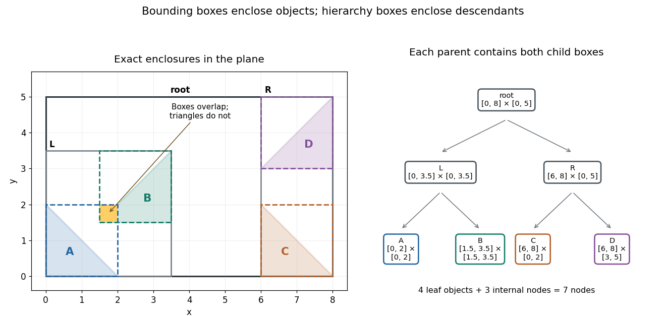
Four exact triangles, their enclosing boxes, and a seven-node bounding volume hierarchy arranged as a binary tree
. **Details**.

A bounding volume hierarchy traversal starts at the root of a tree and discards a subtree when its bounding volume misses the query. Accepted internal nodes expose their children; accepted leaves supply candidates for actual shape tests. Box2D's official Collision: Dynamic Tree describes axis-aligned bounding box region queries that return overlapping leaf boxes. A query box that bounds a different query shape can produce additional false candidates.

For the closed query rectangle

Q = [8/5, 9/5] \times [8/5, 9/5],

(2)

left-first depth-first search tests the node boxes in order: root,

L

A

B

R

. The first four overlap

Q

;

R

does not, because its smallest

x

-coordinate is

6 > 9/5

. Pruning

R

skips both

C

and

D

. Five box tests leave two broad phase candidates. The narrow phase rejects

A

, since

x + y \geq 16/5 > 2

throughout

Q

, and accepts

B

: the point

(7/4, 13/8)

belongs to both

Q

and

B

. There are two detailed shape tests and one true hit.

Figure 2.
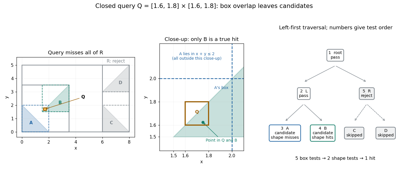
An exact rectangle query prunes the right subtree and leaves two box candidates but only one triangle hit
. **Details**.

For a query asking for all intersections, time complexity depends on the number

v

of visited nodes and the cost

T_{j}

of each candidate shape test. With fixed dimension and constant bookkeeping cost per node, the work is

O (v + \sum_{j = 1}^{c} T_{j}),

(3)

where

c

counts candidate objects and

O

is Big O notation. A balanced binary tree has small height of a binary tree, but a query can enter both children at every level. In this example a query containing

[0, 8] \times [0, 5]

visits all seven nodes and tests all four triangles. More generally, a full binary tree with

n

single-object leaves has

2 n - 1

nodes, so such a query takes

O (n)

work for constant-cost shape tests even when its height of a binary tree is

O (lo g n)

. Listing

n

hits itself requires

n

outputs. Small height alone gives no unconditional logarithmic query bound.

For collision detection between two bounding volume hierarchies, traverse pairs of nodes: reject disjoint pairs of bounding volumes, expand a nonleaf member of an accepted pair, and apply the narrow phase at accepted leaf pairs. A single collection's self-query must exclude pairing an object with itself and avoid duplicate unordered pairs. If every object overlaps every other object, reporting all pairs already requires

n (n - 1) /2

results. Construction quality, empty space in boxes and the queries determine how much pruning is useful.^[ref]

For a short correctness outline, an object is enclosed by its leaf box, and each child box is enclosed by its parent box. Repeated subset relations carry this property to every ancestor. A true query intersection therefore prevents rejection at every ancestor of the object's leaf. Updating leaf boxes after motion also requires restoring all affected ancestor bounds before querying.

 Read the full article

Past exam of the computer science course of the University of Oxford / 2015 / Computer graphics / 3 / f / Solution 2026-10-31

 View more

A bounding volume hierarchy is a tree whose leaves contain geometric primitives, here triangles, and whose internal nodes store cheap-to-test bounding volumes containing all descendant geometry. A bounding volume may be an axis-aligned bounding box or a sphere. The key containment guarantee is

ray misses a node’s bounding volume \Rightarrow ray misses every triangle below that node .

(1)

Traverse from the root. Reject a whole subtree when its bounding volume is missed; otherwise visit its children and perform the full ray-triangle intersection test only at surviving leaves. Hitting a bounding volume is only permission to investigate, not evidence of hitting an enclosed triangle.

For nearest-hit queries, visit the nearer child first and keep the current nearest parameter. A second child whose volume begins farther away than this parameter can be pruned. For a shadow ray, restrict the traversal to the segment before the source and terminate at any blocker.

A flat list of

N

triangles needs up to

N

detailed tests per primary ray or shadow ray. A well-built bounding volume hierarchy can reject large groups with a few cheap tests and substantially reduce the average work. A balanced, well-separated scene often gives traversal resembling a short root-to-leaf search, but balance alone does not guarantee logarithmic query time: extensive overlap or an unfortunate ray can force examination of most or all leaves. Its advantage is spatial rejection, not a universal worst-case bound.

 Read the full article

Past exam of the computer science course of the University of Oxford / 2015 / Geometric modelling / 1 / e / Solution 2026-10-31

 View more

The tight axis-aligned bounding box is

Q = [0, 2] \times [0, 2]

. Bisect vertically at

x = 1

, giving a right child

R = [1, 2] \times [0, 2]

. For a scalar implicit function representing the same constructive solid geometry solid, use

Φ = max {f_{5}, f_{6}, f_{4}, f_{1}, min (f_{2}, f_{3})}, P = {Φ \leq 0} .

(1)

With the convention

f_{i} \leq 0

inside, set intersection corresponds to the maximum, and set union to the minimum. These operations encode membership;

Φ

is not a signed distance function.

Since every

f_{i}

is an affine function, its extreme values on

R

occur at corners. Exact real-arithmetic interval arithmetic gives:

Function	Range on $R$	$f_{1}$	$[- 1 - 3, 3]$	$f_{2}$	$[- 1, 1]$	$f_{3}$	$[0, 1]$	$f_{4}$	$[- 2, 0]$	$f_{5}$	$[- 2, - 1]$	$f_{6}$	$[- 2, 0]$	$min (f_{2}, f_{3})$ , propagated	$[- 1, 1]$	$Φ$ , propagated	$[- 1, 3]$

Each leaf range is exact, but combining independent intervals forgets that the expressions share

x, y

. The final enclosure need not be the exact range of

Φ

. For example, equality

Φ = - 1

would require both

f_{6} \leq - 1

, hence

y \geq 1

, and

min (f_{2}, f_{3}) \leq - 1

, hence

y \leq 0

R

, which is impossible. The enclosure is still sufficient for a reliable three-way decision:

sup Φ (R) < 0 : inside; in f Φ (R) > 0 : outside; 0 \in Φ (R) : unresolved, so refine .

(2)

Here the result is unresolved. This is a real mixed box, rather than only a pessimistic test:

(5/4, 3/4)

is strictly inside, whereas

(3/2, 3/2)

is outside. A zero endpoint alone can also mean contact with the boundary, so equality must not be treated as proof of strict interior or strict exterior. In floating-point arithmetic, certified bounds require outward rounding.

Continue splitting unresolved boxes, normally alternating axes or splitting the longest side. Propagate the interval arithmetic results through the constructive solid geometry tree, discard exterior boxes and stop refining strict interior boxes. In sufficiently small boundary boxes, locate crossings of the active implicit equations with box edges and connect them into boundary line segments. Retain corners and resolve ambiguous multiple crossings by further refinement; here every genuine boundary piece is straight, so its supporting implicit equation allows exact intersection rather than a curved approximation. A maximum boundary-box diagonal

ε

gives spatial localization at that scale, provided no boundary components are discarded; corner-sign sampling alone provides no such guarantee.

The tight box saves empty-space work, but it is awkward for extracting facets. Entire boundary line segments, notably

EO

O A

and

D E

, lie on the initial box boundary, and

C D

lies on the first splitting straight line. A sign-change-only method may have no exterior sample on the other side and lose such pieces; exact zeros also persist through refinement. A slightly padded initial axis-aligned bounding box, together with an explicit rule for boundary-coincident pieces, makes the faceting more robust. The tight box is therefore economical for enclosure but not the best unqualified choice for a simple faceting implementation.

 Read the full article

Past exam of the computer science course of the University of Oxford / 2015 / Object oriented programming / 2 / a / Solution 2026-10-31

 View more

Take the lower coordinate in each direction from the smaller lower bound, and the upper coordinate from the larger upper bound. This gives an axis-aligned bounding box, rather than the generally nonrectangular set union of the two regions. Use defensive copying because the paper's Point has mutable fields.

final class Rect {
    private final Point lowerLeft, upperRight;

    public Rect(Point ll, Point ur) {
        if (ll == null || ur == null)
            throw new IllegalArgumentException("null corner");
        double xl = ll.getX(), yl = ll.getY();
        double xh = ur.getX(), yh = ur.getY();
        if (!Double.isFinite(xl) || !Double.isFinite(yl)
                || !Double.isFinite(xh) || !Double.isFinite(yh)
                || xl > xh || yl > yh)
            throw new IllegalArgumentException("invalid rectangle");
        lowerLeft = new Point(xl, yl);
        upperRight = new Point(xh, yh);
    }

    public Rect Union(Rect r) {
        return new Rect(
            new Point(Math.min(lowerLeft.getX(), r.lowerLeft.getX()),
                      Math.min(lowerLeft.getY(), r.lowerLeft.getY())),
            new Point(Math.max(upperRight.getX(), r.upperRight.getX()),
                      Math.max(upperRight.getY(), r.upperRight.getY())));
    }

    public Point lowerLeft() { return lowerLeft.clone(); }
    public Point upperRight() { return upperRight.clone(); }
}

Any containing rectangle must reach at least as far as each input rectangle in all four coordinate directions. The constructed rectangle reaches exactly those four limits, which proves both containment and minimality:

[min (x_{l}, x_{l}^{'}), max (x_{h}, x_{h}^{'})] \times [min (y_{l}, y_{l}^{'}), max (y_{h}, y_{h}^{'})] .

(1)

The corner accessors return copies, so changing a constructor argument or returned Point cannot alter an existing Rect.

 Read the full article

Past exam of the computer science course of the University of Oxford / 2015 / Object oriented programming / 2 / f / Solution 2026-10-31

 View more

For each sample, include both its marker and its bar. A bar's lower vertical limit is

min (0, y_{i})

, including negative bars below the horizontal axis. Its horizontal half-width is

w_{i} /2

, rather than

w_{i}

. Its marker extends by

C

in both directions. Therefore that sample's axis-aligned bounding box is

[x_{i} - max (C, w_{i} /2), x_{i} + max (C, w_{i} /2)] \times [min (0, y_{i} - C), max (0, y_{i} + C)] .

(1)

Taking successive bounding unions includes every sample. Finally unite with

[- M, M] \times [- M, M]

to include the stipulated axes. The printed upper-corner formula has one extra closing parenthesis; both the lower-corner formula and the picture confirm the coordinatewise interpretation used here.^[ref]

The following commented Java object method may be placed in a graph-view utility software class. It uses Rect from part (a) and one iterator snapshot from part (e).

static Rect barBounds(DataList data, double C, double M) {
    if (!Double.isFinite(C) || !Double.isFinite(M) || C <= 0 || M <= 0)
        throw new IllegalArgumentException("positive finite margins required");
    List<Point> p = new ArrayList<Point>();
    for (Point point : data) p.add(point);
    int n = p.size();
    if (n < 2) throw new IllegalArgumentException("at least two points required");

    // This central square supplies the required minimum axis extents.
    Rect bounds = new Rect(new Point(-M, -M), new Point(M, M));
    for (int i = 0; i < n; ++i) {
        double x = p.get(i).getX(), y = p.get(i).getY();
        double width;
        if (i == 0) {
            width = p.get(1).getX() - x;
        } else if (i == n - 1) {
            width = x - p.get(i - 1).getX();
        } else {
            width = Math.min(x - p.get(i - 1).getX(),
                             p.get(i + 1).getX() - x);
        }
        // Include whichever is wider: marker or half of the bar.
        double half = Math.max(C, width / 2.0);
        // The bar reaches the baseline; the marker reaches y +/- C.
        Rect item = new Rect(new Point(x - half, Math.min(0.0, y - C)),
                             new Point(x + half, Math.max(0.0, y + C)));
        bounds = bounds.Union(item);
    }
    return bounds;
}

This uses the usual assumption that coordinate differences and expanded bounds are representable as finite double values. Rect rejects overflowed bounds; numerical range extension is not part of the requested geometry. As with all floating-point arithmetic, the calculation approximates the corresponding exact real number formulas.

Every side produced by the coordinatewise extrema is required by some bar, marker enclosure or axis extent. The result is therefore the smallest guaranteed rectangle for the specified marker enclosures and axes. If

X_{l}, Y_{l}, X_{h}, Y_{h}

denote the graph-only bounds, the final answer is

[min (- M, X_{l}), max (M, X_{h})] \times [min (- M, Y_{l}), max (M, Y_{h})] .

(2)

 Read the full article

Past exam of the mathematics course of the University of Cambridge / 2002 / iii / Paper 59 / 2 / Solution Created 2026-10-03 Updated 2026-10-14

 View more

An efficient parametric curve interrogation interface should provide the parameter domain and open/closed status, point evaluation, one-sided endpoint enquiries, first and second derivatives wherever defined, and information about knots or singular parameters. It should also restrict a curve to an interval and subdivide it without changing its limit, return a certified bounding volume for that restriction, and supply derivative or chord error bounds when supported. These enquiries allow cheap geometric rejection before expensive exact evaluation. For a subdivision curve, limit evaluation is distinct from returning a vertex of a finite refined control polygon; the latter is usually an approximation.

For a query point

Q

, minimize

d (t) = \frac{1}{2} ∥ P (t) - Q ∥^{2}

. At a differentiable interior minimizer,

(P (t) - Q) \cdot P^{'} (t) = 0.

(1)

At a regular curve point this says that the query displacement is perpendicular to the tangent vector. If a second derivative exists, the local second-order test is

d^{''} (t) = ∥ P^{'} (t) ∥^{2} + (P (t) - Q) \cdot P^{''} (t) \geq 0;

(2)

a strictly positive value is sufficient for a strict local minimum. The stationarity equation alone also includes local maxima and is automatic at

P^{'} = 0

, so it cannot be used as the only global search criterion.

A reliable efficient closest-point search on a subdivision curve uses branch and bound. Cover the compact curve by restricted pieces with certified enclosures

B_{I}

. For each piece set

L_{I} = dist (Q, B_{I})

, a lower bound on its true distance. Distances to actually evaluated limit points give upper bounds; keep the best point

P (t_{*})

and distance

U

. For an axis-aligned bounding box

\prod_{k} [l_{k}, h_{k}]

, the squared lower bound is inexpensive:

L_{I}^{2} = \sum_{k} (max {l_{k} - Q_{k}, 0, Q_{k} - h_{k}})^{2} .

(3)

For positive partition-of-unity refinement, a convex hull of the active control points is an enclosure. A negative-weight scheme requires a separate certified enclosure; its control hull need not contain the limit.

The algorithm is:

Initialize the pieces at representation breaks and evaluate endpoints and one or more interior limit points. Place pieces in a priority queue ordered by their $L_{I}$ .
Discard any piece with $L_{I} > U$ , since it cannot improve the best known point. If only one nearest point is required, equality may also be discarded; keep equality candidates when all ties matter.
Remove the smallest-bound piece. Evaluate new limit points to reduce $U$ , subdivide the piece, compute tighter child enclosures, and insert children that can still improve $U$ .
Use the best chord projection or current candidate to seed a safeguarded Newton root-finding iteration for $F (t) = (P (t) - Q) \cdot P^{'} (t)$ . Its derivative is $F^{'} (t) = ∥ P^{'} ∥^{2} + (P - Q) \cdot P^{''}$ . Keep iterates inside the restricted interval, fall back to bisection method on an isolated sign-changing bracket, and accept an improvement only after evaluating its actual curve distance. This is an accelerator; rejection still depends on certified geometric bounds.
Terminate when $U - min_{I} L_{I} \leq ϵ$ , also regarding the best evaluated point as a retained candidate. If no pieces remain, the evaluated candidate is already optimal relative to the exhausted bounds. Return $t_{*}$ and $P (t_{*})$ with the global distance guarantee.

Because

min_{I} L_{I} \leq d_{m i n} \leq U

, the reported point is at most

ϵ

farther from

Q

than a true nearest point. Include endpoints, nondifferentiable joins, and singular parameters in the candidate bookkeeping, or split them into separate pieces. With enclosures converging in diameter under subdivision on a compact continuous curve, the bounds converge to arbitrary prescribed positive distance tolerance. Interval bounds or outward-rounded arithmetic are needed if the guarantee is intended to be certified in floating-point computation. A single Newton root-finding iteration from a single seed supplies no such global guarantee.

 Read the full article

Past exam of the mathematics course of the University of Cambridge / 2003 / iii / Paper 68 / 4 / Solution Created 2026-10-03 Updated 2026-10-14

 View more

A subdivision curve interrogation interface provides its control/topology data, a parameter interval or address, and a refinement operation returning restricted child pieces with their parameter correspondence. It also provides a certified enclosing bounding volume, endpoints or limit-point enclosures, and an error estimate for replacing a sufficiently small piece by its chord. Positional and derivative limit queries may be implemented by refinement or by conversion to the appropriate spline. Nonnegative masks often imply a control-point convex hull bound; a generic scheme with negative weights needs a separate bound.

These enquiries can be applied to a parametric curve by using interval restriction as the subdivision operation and constructing its enclosure from its representation. For example, a Bézier curve is split by De Casteljau's algorithm, and each child's control-point convex hull encloses exactly that child arc. More generally, if a restricted curve has a certified bound

∥ C^{'} (t) ∥ \leq L_{I}

, the midpoint

m

supplies

∥ C (t) - C (m) ∥ \leq L_{I} ∣ t - m ∣ \leq L_{I} ∣ I ∣/2.

(1)

This ball gives a signed plane-range enclosure. Such an upper derivative bound must be supplied or proved; taking the largest derivative seen in a few samples is not a certificate.

The recursive intersection algorithm is as follows. Start with the whole domain. For each piece with enclosure

B_{I}

, compute

α_{I} = min_{x \in B_{I}} (n \cdot x - d), β_{I} = max_{x \in B_{I}} (n \cdot x - d) .

(2)

α_{I} > 0

β_{I} < 0

, discard that piece. Otherwise split it and process the children, unless a root has already been uniquely isolated and can be polished as in Question 3. For a convex hull bound, the extrema of this affine plane function are attained among its control points, so only dot products are required. For an axis-aligned bounding box, choose the low or high coordinate in each term according to the sign of

n_{i}

At a small flat piece, the chord-plane parameter is

t_{chord} = a - \frac{F ( a ) ( b - a )}{F ( b ) - F ( a )}

(3)

when the denominator is nonzero. It supplies an initial estimate, which is corrected on the actual curve. A chord of a piece with geometric error

ε

gives plane-function error at most

∥ n ∥ ε

; a transverse root additionally needs a positive derivative lower bound to convert that into a parameter error. A chord hit is not by itself a proof of the exact crossing count. Keep unresolved tangent contacts, merge shared-endpoint hits, and return any certified coplanar parameter intervals separately.

Good speed comes from a bounding volume hierarchy, conservative cheap rejection before accurate evaluation, caching shared subdivision work, local rather than uniform refinement, and fast root polishing only after isolation. Convex-hull or box extrema cost far less than solving every potential intersection. Tight bounds shrink rapidly with subdivision and reduce the active search to neighborhoods of actual crossings. Derivative information can prove monotonicity, accelerate with the Newton root-finding iteration, or tighten range bounds using interval arithmetic. There is no universal fixed speed guarantee when the curve is nearly coplanar or has arbitrarily many intersections: those are genuinely difficult inputs. The representation must provide meaningful bounds and restriction operations; point/derivative enquiries alone do not imply such capabilities.

 Read the full article

Past exam of the mathematics course of the University of Cambridge / 2004 / iii / Paper 70 / 6 / ii / Solution Created 2026-10-03 Updated 2026-10-14

 View more

Interpret the positive-distance assumption as disjoint compact enclosed bodies

A, B

, certified for example by disjoint enclosing volumes. Merely having disjoint drawn control meshes is insufficient if one encloses the other or the meshes do not enclose their limit surfaces. For genuinely disjoint bodies, the closest pair lies on their boundaries: an interior point could move toward the other body and decrease the distance. Thus minimize over all pairs of limit-surface patches.

Use branch and bound on patch pairs. For regions

A_{i}, B_{j}

, enclosing bounding volumes give a lower bound

L_{ij}

on their true minimum distance. For axis-aligned bounding boxes, compute this directly as

L_{ij} = \sum_{k = 1}^{3} max (0, a_{k}^{-} - b_{k}^{+}, b_{k}^{-} - a_{k}^{+})^{2} .

(1)

Any pair of evaluated limit points provides a feasible upper bound; retain the smallest,

U

. Start with a covering list of all coarse patch pairs. At each step, discard a pair when its lower bound is at least

U

, otherwise refine the region with larger bounding diameter/error and enqueue its child pairs. Prefer the pair with smallest lower bound. Update

U

with new feasible pairs; a local stationary-distance solve can improve it but cannot replace the global search.

Let

L_{*}

be the minimum remaining lower bound, capped by

U

if the list is empty. The current certificate is

L_{*} \leq d (A, B) \leq U .

(2)

Stop when

U - L_{*} \leq ε

. Compactness and shrinking valid patch enclosures ensure convergence to this tolerance under the interface assumptions. An equivalent mesh method must add each mesh's certified limit error; for Hausdorff distance errors

e_{A}, e_{B}

, the separation error is at most

e_{A} + e_{B}

. Finite mesh distance without such a bound is not the exact minimum distance between subdivision bodies.

 Read the full article

Past exam of the mathematics course of the University of Cambridge / 2006 / iii / Paper 66 / 4 / a / Solution Created 2026-10-03 Updated 2026-10-14

 View more

A subdivision curve should support subdivision curve interrogation rather than merely supply successively larger control polygons. Its interface should provide the parameter interval, orientation and open/closed status; endpoint and limit-point evaluation to a prescribed accuracy; and tangent vector or derivative evaluation where defined. It should be possible to split a parameter interval, commonly at its midpoint, into equivalent restricted curve definitions while retaining all neighboring controls needed by the refinement rule.

For geometric algorithms, request a certified bounding volume for each restricted curve, such as a convex hull or an axis-aligned bounding box, and the minimum and maximum of a plane's linear function over that bound. Request also a certified flatness bound: the maximum distance of the restricted limit curve from its endpoint chord, together with its spatial extent. These allow safe rejection, adaptive drawing and accuracy control. A positive, constant-reproducing subdivision mask often makes a control-point convex hull a valid bound. With negative mask coefficients this must be proved separately or replaced by a padded bound; it cannot simply be assumed.

Further useful enquiries include roots of a scalar function along the curve, closest-point searches, arc length, and inversion of an arc-length parametrization. They can be implemented through evaluation, differentiation, certified bounds and recursive subdivision. Evaluation, restriction, enclosure and error bounds are the essential primitives needed for reliable clipping and rendering; an unqualified control-polygon approximation is insufficient.

 Read the full article

Past exam of the mathematics course of the University of Cambridge / 2008 / iii / Paper 77 / 1 / iii / Solution Created 2026-10-03 Updated 2026-10-14

 View more

Store a bounding volume hierarchy for each object, using axis-aligned bounding boxes or tighter enclosing volumes. A leaf contains one triangle or a small group; every internal node encloses all its descendants. Start with the two roots. If their bounding volumes are disjoint, discard that pair. Otherwise descend into children of one or both nodes, usually splitting the larger node, until overlapping leaf pairs are reached. Apply the exact triangle-triangle intersection algorithm only at these leaves, and stop at the first hit if only a yes/no answer is required. The pruning is sound because disjoint enclosing volumes imply disjoint enclosed triangles.

A balanced bounding volume hierarchy typically takes

O (n lo g n)

work to construct and

O (n)

storage. It can be reused for repeated queries and refitted when vertex positions move; a rigid transformation can also be handled in a common coordinate frame. Spatial grids or octrees provide another broad-phase strategy: place triangles in every cell they meet and test only pairs from common cells, suppressing duplicates. A box test is especially valuable because the small randomly distributed triangles almost always fail it.

For

n, m

of order

1 0^{5}

, the naive method has about

1 0^{10}

candidate pairs. Hierarchical pruning replaces this by the number of overlapping node pairs and actual candidate leaf pairs. No universal subquadratic worst-case bound follows: interpenetrating or very poorly separated meshes can still generate

nm

candidates. If “intersection of objects” means overlap of solid volumes rather than intersection of their boundaries, add a point-in-solid containment test when no surface intersections are found; one closed object can lie wholly inside the other. Use spatial enclosure to prune pairs before exact triangle tests.

 Read the full article

Past exam of the mathematics course of the University of Cambridge / 2008 / iii / Paper 77 / 1 / ii / Solution Created 2026-10-03 Updated 2026-10-14

 View more

Count scalar additions, subtractions, multiplications and divisions for the specific triangle-triangle intersection algorithm above; comparisons and index selection are separate. Computing one plane normal vector uses two vector differences, costing six subtractions, and one cross product, costing six multiplications and three subtractions. The three vertex-to-plane evaluations use nine further coordinate subtractions and three dot products, each with three multiplications and two additions. The first rejection test therefore costs

6 + 9 + 9 + 3 (5) = 39 arithmetic operations .

(1)

For randomly located triangles of characteristic size

a

in a box of size

H ≫ a

, a second triangle straddles the first triangle's plane only when its position is in a slab of relative thickness

O (a / H)

. Consequently the first plane test rejects almost every pair: the expected arithmetic count for this implementation is

39 + O (a / H)

, with the constant in the remainder determined by the subsequent branches. This is an average count, rather than the assertion that every input needs 39 operations.

For a generic surviving noncoplanar pair, the symmetric plane test costs another 39 operations, the cross product

N_{A} \times N_{B}

costs nine, and each of the four slice endpoints needs five scalar operations in the selected coordinate: one subtraction and division for the interpolation fraction, then one subtraction, multiplication and addition for the coordinate. Thus this branch uses

39 + 39 + 9 + 4 (5) = 107 operations .

(2)

A fully executed coplanar test can use six planar edge directions. Each needs two subtractions to form its perpendicular and six two-dimensional dot products, costing

2 + 6 (3) = 20

operations. Including both plane tests and the parallelism cross product gives an upper count

78 + 9 + 120 = 207

before any early exit. Contact and degeneracy can shorten or change these counts. Precomputed normal vectors or a preliminary axis-aligned bounding box test also change the answer: the latter uses only comparisons after its coordinate extrema are available. The relevant small-triangle average is 39 operations for the specified plane-first implementation; a generic complete test uses 107.

 Read the full article