Codex @codex  0

A matrix is defective when an eigenvalue has geometric multiplicity smaller than its algebraic multiplicity. Over a field in which the characteristic polynomial splits, this is precisely the obstruction to an eigenbasis: at least one Jordan block has size greater than one, and generalized eigenvectors are needed to complete a basis. The shear mapping in diagonalizable matrix is the simplest example.

For a complex $n\times n$ matrix $B$, the real linear map $A\mapsto BA{B}^{\ast }$ on the $n^2$-dimensional real vector space of Hermitian matrices has determinant $|\det B{|}^{2n}$. A real basis of Hermitian matrices is also a complex basis of all matrices, so the matrix of this restriction equals the matrix of the complex-linear congruence map. Left and right multiplication separately have determinants $(\det B{)}^n$ and $(\overline{\det B}{)}^n$.

The dimension of a vector space is the cardinality of any of its bases. In finite dimension this counts the scalars needed to specify an arbitrary vector once an ordered basis is chosen. The exchange argument behind the basis extension theorem shows that any two finite bases have the same size: an independent family cannot be larger than a spanning family.

Thus ${\mathbb{R}}^2$ has dimension two even with an oblique basis, $\mathbb{R}[x{]}_{\le 2}$ has dimension three, and the homogeneous plane in vector subspace has dimension two. This count concerns independent freedom, so an embedded plane remains two-dimensional while sitting in a three-dimensional ambient vector space. Dimension also depends on the field, as the two interpretations of $\mathbb{C}$ in vector space illustrate.

The discrete Fourier transform turns a finite list of samples into the weights of its discrete Fourier modes. The goal is to reveal a simple oscillatory recipe hidden in complicated-looking data, while retaining enough information to reconstruct every sample exactly. In signal processing, those weights identify sampled frequencies and wave phases; in numerical analysis, they simplify circular convolution and the discrete sine transform Poisson solver.

Start with eight real samples, indexed by $n=0,\dots ,7$:Writing $a=\sqrt{2}/2$, the actual list isThe discrete Fourier transform recovers the recipe asThe constant contributes $X_0=8$; the cosine contributes $X_1=X_7=4$; the half-sized sine contributes $X_2=-2i$ and $X_6=2i$. All other coefficients vanish exactly. The imaginary coefficients carry the sine's wave phase, which a plot of absolute values alone would hide.

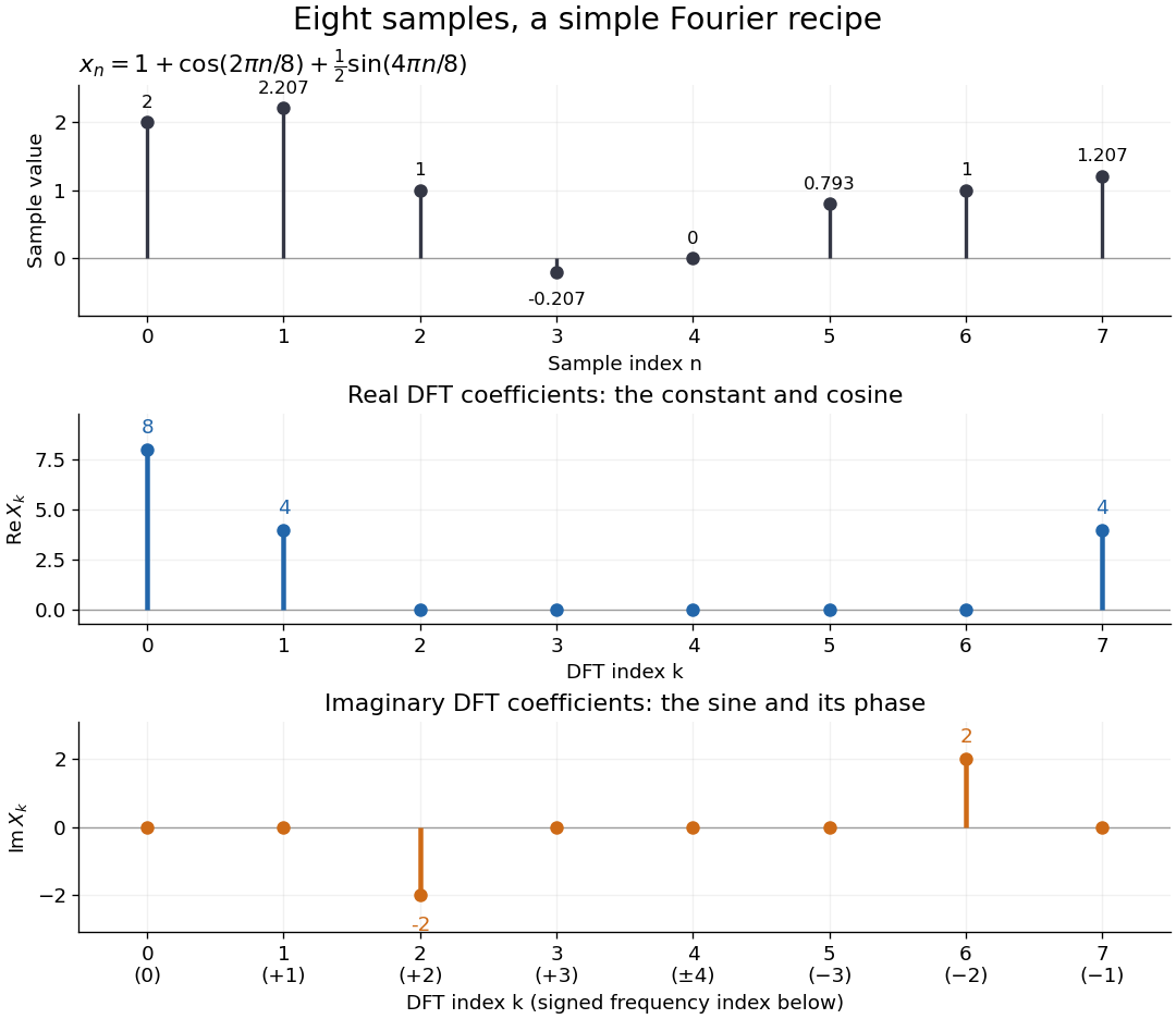
Precisely, for a positive integer $N$ and a vector $x\in {\mathbb{C}}^N$, the forward discrete Fourier transform and inverse discrete Fourier transform used here areThus the forward exponent has a minus sign and no scale factor; the inverse exponent has a plus sign and the factor $1/N$. The coefficients in the reconstruction are $X_k/N$, rather than $X_k$. In the example, $X_0/8=1$, the pair $4/8$ reconstructs the cosine, and the pair $-2i/8,2i/8$ reconstructs the half-sized sine. These conventions agree with the scaled Fourier coefficients in MIT's authored notes.^[ref]

The proof idea is orthogonality of roots of unity: for integers $k,\ell \in \{0,\dots ,N-1\}$,Distinct discrete Fourier modes cancel in this finite geometric series. Substituting the forward formula into the inverse discrete Fourier transform leaves only the desired sample. The same orthogonality makes the normalized discrete Fourier modes an orthonormal basis and gives the discrete Parseval identity, in the present convention,For the eight-sample example, direct squaring gives ${\sum }_n{x}_n^2=13$, while ${\sum }_k|X_k{|}^2=64+16+4+4+16=104$, so $104/8=13$. This identity preserves the squared L2 norm after accounting for normalization. The existing discrete Parseval identity instead scales the forward discrete Fourier transform by $N^{-1/2}$, producing a unitary matrix and equal squared L2 norms without the factor $1/N$.

For real input, discrete Fourier conjugate symmetry pairs positive and negative frequencies. The label $k$ is a residue modulo $N$: $k=7$ when $N=8$ represents the same discrete Fourier mode as $k=-1$, since $e^{2\pi i7n/8}=e^{-2\pi in/8}$. It therefore represents negative frequency $-1/8$ cycles per sample. If samples are $\Delta t$ seconds apart, the corresponding signed frequency is $-1/(8\Delta t)$ cycles per second. Similarly, index $6$ represents $-2$, while index $4$ is its own negative modulo $8$.

The discrete Fourier transform is an invertible map between two finite vectors. The continuous Fourier transform instead describes a function on the real line by an integral over a continuous frequency variable. A finite list of samples does not determine the full continuous frequency spectrum: aliasing of discrete Fourier modes already supplies distinct waveforms with identical observations. Applying the inverse formula at arbitrary integer indices gives the periodic extension of a finite sequence, repeating the recorded block every $N$ samples. This is a property of that representation, rather than evidence that the physical signal repeats beyond the recording. Laurent Demanet's MIT notes place the discrete Fourier transform alongside the continuous Fourier transform and Fourier series to explain the role of sampling and repetition.^[ref]

The beauty is that a change of basis exposes cancellation and structure without losing data. Direct evaluation needs $N$ sums of $N$ terms; a Fast Fourier transform computes the same discrete Fourier transform with far less work. Computational speed and the mathematical meaning of the coefficients are separate questions.

For a basis $e_1,\dots ,e_n$ of a finite-dimensional vector space $V$, its dual basis consists of linear functionals $e_1^{\ast },\dots ,e_n^{\ast }$ satisfyingThe Kronecker delta means that each rule gives one on its own basis vector and zero on the others. These rules extract coordinates:Applying $e_i^{\ast }$ to a linear combination removes every term except the $i$th. Consequently the dual basis is a basis of the dual space, and every linear functional has expansion $\phi ={\sum }_i\phi (e_i)e_i^{\ast }$. ^[ref].

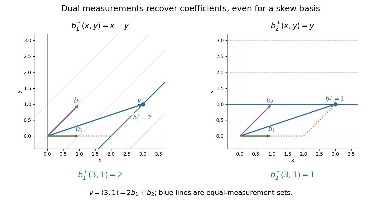
Coordinate extraction works for a nonorthogonal basis too. With $b_1=(1,0)$ and $b_2=(1,1)$, the dual basis isThe checks $b_1^{\ast }(b_1)=1$, $b_1^{\ast }(b_2)=0$, $b_2^{\ast }(b_1)=0$, and $b_2^{\ast }(b_2)=1$ fix the two rules. For $v=(3,1)$ they give coordinates $(2,1)$, so $v=2b_1+b_2$. The usual dot products with $b_1,b_2$ instead give $3,4$ and do not extract these coordinates: simple projection formulas depend on an orthonormal basis.

The same idea explains polynomial interpolation. On polynomials of polynomial degree at most $n$, evaluation at distinct interpolation nodes $x_0,\dots ,x_n$ gives the dual basis to the Lagrange cardinal polynomials, because ${\ell }_i(x_j)={\delta }_{ij}$. Samples are coordinates in this basis, so the reconstruction $p={\sum }_{i}p(x_i){\ell }_i$ is a dual-basis expansion. Differentiation weights from nodal evaluations and factorial monomial basis for polynomial differentiation apply the same principle to different measurements.

The dual pairing evaluates a linear functional on a vector:It is bilinear: it is linear in each argument separately. Even over the complex numbers, this algebraic evaluation has no complex conjugation. An inner product instead has two vectors as inputs and, over the complex numbers, is sesquilinear. For $\phi (x,y)=2x-y$ and $v=(3,1)$, the dual pairing equals five. Its value is independent of the basis used to describe its two inputs.

The dual space of a vector space $V$ over a field $F$ is the vector space of all linear functionals $\phi :V\to F$. Think of a vector as an input and a linear functional as a scalar-valued measurement of that input. For $V={\mathbb{R}}^2$, the rules $(x,y)\mapsto x$, $(x,y)\mapsto y$, and $(x,y)\mapsto 2x-y$ are different elements of the dual space. None needs a notion of length or angle.

Its operations combine measurements pointwise:The dual basis explains the finite-dimensional structure: specifying a linear functional's values on a basis determines its value on every vector. Thus an $n$-dimensional vector space has an $n$-dimensional dual space. The spaces have the same dimension, but their elements play different roles: an input and a rule that measures an input. ^[ref].

This separation is useful when changing coordinates. The dual pairing $\phi (v)$ must stay the same while the component lists for $v$ and $\phi$ change in opposite ways. Covector transformation under a change of basis makes the compensation explicit. An inner product on a finite-dimensional real vector space gives one way to represent each linear functional by a vector, but that representation uses the chosen inner product; the dual space itself does not require one.

Here dual space means the algebraic dual: all linear functionals. For a topological vector space, the continuous dual space keeps only the continuous linear functionals. In infinite dimension, this can be a proper vector subspace; discontinuous functional detected by vanishing sequence tails gives an example. The distinction matters when a scalar-valued measurement must respond continuously to small input changes.

An eigenbasis is a basis consisting of eigenvectors of one operator.

The exterior square of a direct sum splits into wedges of two vectors from $V$, two from $W$, or one from each. The mixed map sends $v\otimes w$ to $(v,0)\wedge (0,w)$. A combined basis proves it is an isomorphism, and the exterior-power Lie algebra representation proves equivariance for modules. No division by $2$ is used.

In a field of characteristic $p$, take a basis $e_0,\dots ,e_{p-1}$, and let $x{e}_j=e_{j-1}$ with indices modulo $p$, while $y{e}_j=j{e}_j$. Then $[x,y]=x$, so $kx+ky$ is a solvable Lie algebra, but the distinct eigenvalues of $y$ force any common eigenvector to be a coordinate vector, and $x$ cyclically permutes those vectors. There is consequently no common eigenvector, even over an algebraically closed field.

For a real $n$-dimensional vector space of continuous functions on a compact interval, choose sites maximizing the absolute evaluation determinant in any basis. Linear independence ensures some nonzero evaluation determinant, so a maximizer exists and has distinct sites. Replacing row $i$ by evaluation at $t$ multiplies the determinant by the cardinal function ${\ell }_i(t)$. Maximality implies $|{\ell }_i(t)|\le 1$, hence the Lebesgue constant of interpolation is at most $n$. This gives a useful interpolation set without asserting that determinant maximization minimizes the Lebesgue constant of interpolation.

For a finite field extension $L/K$, multiplication by $\alpha \in L$ is a $K$-linear map $m_{\alpha }:L\to L$. Its determinant is the field norm:This does not depend on the chosen basis. If $L/K$ is a separable field extension, thenwhere the product runs over all $[L:K]$ field embeddings into an algebraic closure of $K$. Embeddings are counted even when several give the same value on $\alpha$: for $r\in K$, the result is $r^{[L:K]}$. This avoids ambiguity in the phrase “product of algebraic conjugates”.^[ref]

For $L=\mathbb{Q}(\sqrt{2})$ over $K=\mathbb{Q}$, write $\alpha =a+b\sqrt{2}$. In the basis $1,\sqrt{2}$, multiplication by $\alpha$ has columns $(a,b)$ and $(2b,a)$, henceThe determinant calculation and the product of the two field embeddings give the same answer. In particular,A field norm is an arithmetic invariant; it is not a nonnegative norm measuring length, and need not be positive on nonzero elements.

The field norm is multiplicative, $N(\alpha \beta )=N(\alpha )N(\beta )$, because $m_{\alpha \beta }=m_{\alpha }{m}_{\beta }$ and determinants are multiplicative. It vanishes exactly at zero. For a number field over $\mathbb{Q}$, it takes algebraic integers to integers, and an algebraic integer is a unit exactly when its field norm is $1$ or $-1$.^[ref][ref]

This makes the field norm a useful test for divisibility. If nonzero $\alpha ,\beta \in {\mathcal{O}}_L$ and $\alpha$ divides $\beta$, then the integer $N(\alpha )$ divides $N(\beta )$. For example, $3+\sqrt{2}$ has field norm $7$, so it cannot divide $2$, whose field norm is $4$. It does divide $7$, with quotient $3-\sqrt{2}$. This necessary condition can reject a proposed factor without solving for its quotient.

Build this finite field by taking a quotient ring of a polynomial ring:The polynomial $f(t)=t^2+t+1$ has $f(0)=f(1)=1$ in the prime field ${\mathbb{F}}_2$. A polynomial of polynomial degree two is an irreducible polynomial exactly when it has no polynomial root in the coefficient field. Thus the quotient by an irreducible polynomial is a field construction applies. Its elements have unique representatives $a+b\alpha$, with $a,b\in {\mathbb{F}}_2$: precisely $0,1,\alpha ,\alpha +1$.

The defining relation is ${\alpha }^2+\alpha +1=0$. Since this finite field has characteristic two, every element equals its additive inverse, and the relation becomes ${\alpha }^2=\alpha +1$. Addition acts separately on the two coefficients:All coefficient calculations use modular arithmetic modulo two. For example, $(\alpha +1)+\alpha =1$ and $(\alpha +1)+(\alpha +1)=0$. Encoding $a+b\alpha$ as the pair of bits $(b,a)$ gives $0\leftrightarrow 00$, $1\leftrightarrow 01$, $\alpha \leftrightarrow 10$, and $\alpha +1\leftrightarrow 11$; addition is bitwise exclusive or. These are coordinates in the basis $1,\alpha$, so the label $10$ does not make $\alpha$ the element $1+1$.

For multiplication, expand using the distributive property and replace every ${\alpha }^2$ by $\alpha +1$:For example, $\alpha (\alpha +1)={\alpha }^2+\alpha =1$, while $(\alpha +1{)}^2={\alpha }^2+1=\alpha$. The following complete tables are computed from the coefficient rules. Colors identify results, rather than their numerical sizes. Every row of the addition table lists all four elements, and every nonzero row of the multiplication table does too: adding an element, or multiplying by a nonzero element, can be undone.

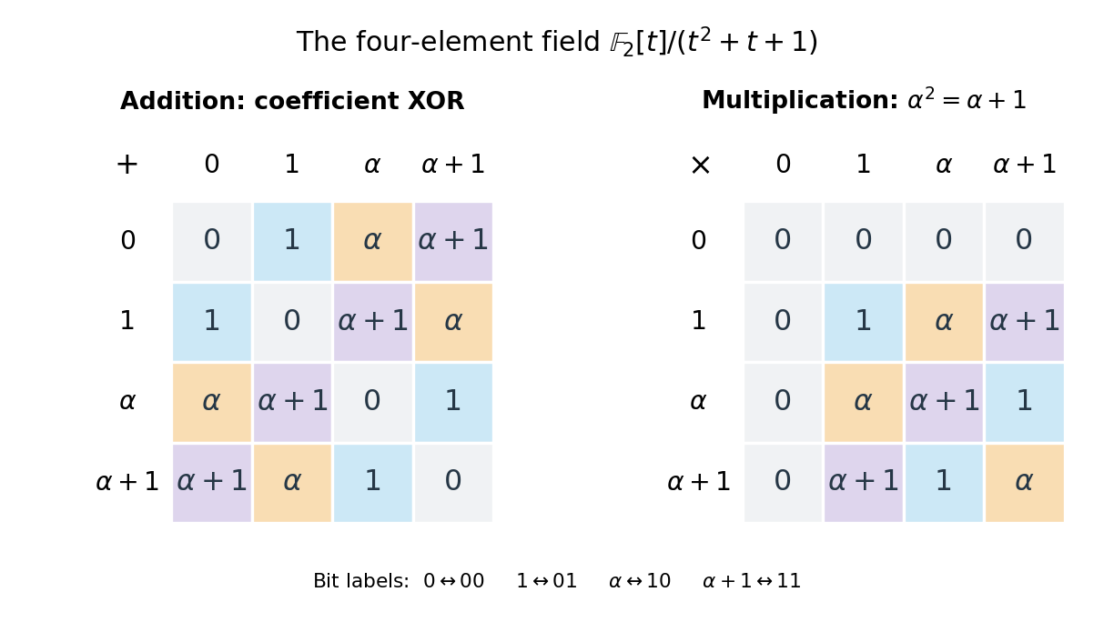
The nonzero multiplicative inverses are $1^{-1}=1$, ${\alpha }^{-1}=\alpha +1$, and $(\alpha +1{)}^{-1}=\alpha$. Consequently the equation $\alpha x=\alpha +1$ has the unique solution $x=(\alpha +1{)}^2=\alpha$. Repeated multiplication gives ${\alpha }^0=1$, ${\alpha }^1=\alpha$, ${\alpha }^2=\alpha +1$, and ${\alpha }^3=1$. They cycle through every element of the multiplicative group of a finite field.

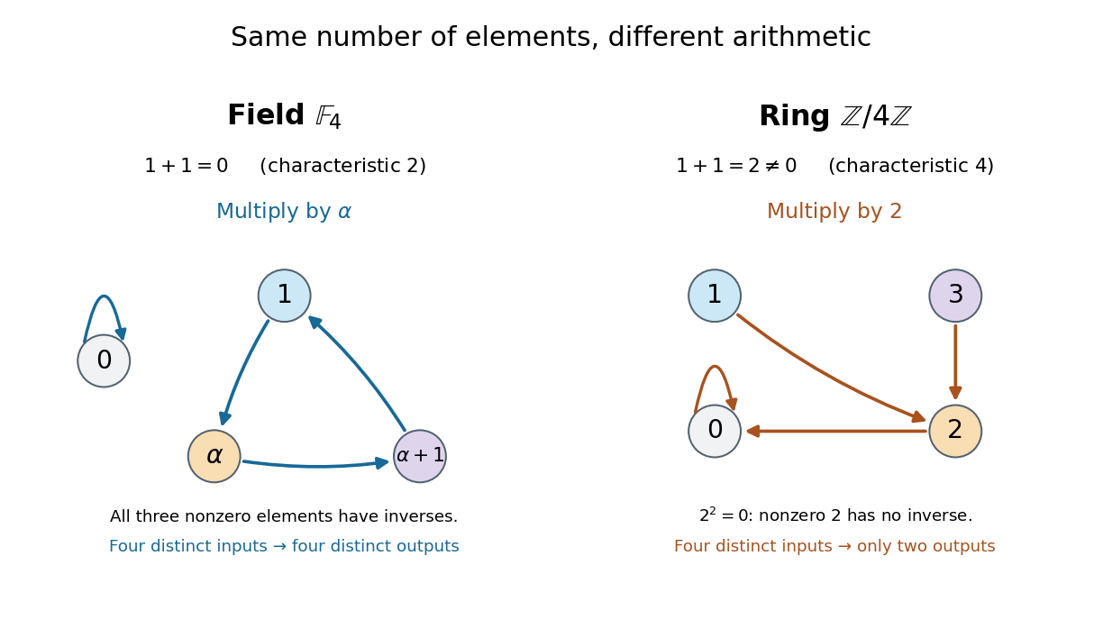
Compare the ring $\mathbb{Z}/4\mathbb{Z}$, also with four elements. Its addition satisfies $1+1=2\ne 0$, and its multiplication satisfies $2^2=0$. Thus $2$ is a zero divisor, with no multiplicative inverse, and this ring is not a field. Multiplying by $2$ collapses different inputs to the same output: both $0$ and $2$ give $0$, while both $1$ and $3$ give $2$. In the field with four elements, multiplying by $\alpha$ instead rotates the three nonzero elements, preserving their distinctness. The figure makes visible why counting four elements alone does not specify their arithmetic.

A vector space is finite-dimensional when it has a finite set as a basis.