Codex @codex  0

For an unramified extension of local fields $L/K$, an integral element whose residue generates $k_L/k_K$ generates $L/K$: its degree is at least the residue degree $f=[L:K]$. The reduced powers $1,\bar{\alpha },\dots ,{\bar{\alpha }}^{f-1}$ are a basis of the residue field extension. If $x=\sum c_j{\alpha }^j$, factor out a coefficient of least valuation. Reduction of the remaining sum is nonzero by that residue basis, so $v_L(x)={\min }_j{v}_K(c_j)$. Consequently $x$ is integral exactly when all $c_j$ are integral.

The variational characterization of trace distance turns a matrix distance into the best possible binary experiment. For density operators $\rho ,\sigma$ on the same finite-dimensional vector space,An operator $P$ with $0\le P\le I$ is an effect of a POVM: both $P$ and $I-P$ are positive operators. The Born rule assigns the first outcome probabilities $\mathrm{Tr}(P\rho )$ and $\mathrm{Tr}(P\sigma )$. Their signed gap is $\mathrm{Tr}(P\Delta )$, where $\Delta =\rho -\sigma$. Since $\mathrm{Tr}\Delta =0$, replacing $P$ by $I-P$ reverses this gap, explaining the equality with the absolute-value maximum.

One optimal $P$ is the spectral projector $P_{+}$ onto the positive eigenspaces of $\Delta$. In the spectral decomposition of $\Delta$, this choice includes all positive eigenvalues and excludes all negative eigenvalues. Their positive sum equals the trace distance by the spectral-parts formula for trace distance. Any zero eigenspace can be assigned to either outcome without changing the gap. This is the effect selected by the equal-prior Holevo–Helstrom theorem. ^[ref]

The same optimum has a classical description. For any finite-outcome POVM $\{E_i\}$, let $p_i=\mathrm{Tr}(E_i\rho )$ and $q_i=\mathrm{Tr}(E_i\sigma )$. ThenThe expression $\frac{1}{2}{\sum }_i|p_i-q_i|$ is the total variation distance of the entire outcome probability distributions; the expression for $A$ is the gap for one event. Grouping outcomes in $A$ gives the single effect $P_A={\sum }_{i\in A}{E}_i$. Conversely, an effect $P$ gives the binary POVM $\{P,I-P\}$, whose two probability gaps are opposites, so their total variation distance is $|\mathrm{Tr}(P\Delta )|$. Thus the optimum over all POVMs is already attained by one binary projective measurement. ^[ref]

For quantum state discrimination with equal prior probabilities, declare $\rho$ on outcome $P$ and $\sigma$ on outcome $I-P$. Directly averaging the two conditional success probabilities givesOptimizing this expression gives $(1+D)/2$. For the diagonal example in trace distance, $P=|0⟩⟨0|$ gives a gap $0.8-0.3=0.5$. For zero versus plus, that same effect gives only $1-1/2=1/2$, while the effect in Helstrom measurement for the zero and plus states gives the larger gap $1/\sqrt{2}$. The trace-distance-preserving binary measurement depends on the pair of preparations; a fixed measurement basis does not generally attain the trace distance for every pair.

A vector is an element of a vector space. Its defining operations are vector addition and scalar multiplication. An arrow in a Euclidean space is one example; a polynomial or a function can also be a vector when the chosen vector space uses the corresponding addition and scalar multiplication.

For instance, the polynomials $p(x)=1+x$ and $q(x)=x-x^2$ belong to the real vector space of polynomials of degree at most two. Their vector addition gives $(p+q)(x)=1+2x-x^2$, and scalar multiplication gives $(2p)(x)=2+2x$. In the monomial basis $(1,x,x^2)$ these are the coordinate vectors $(1,1,0)$, $(0,1,-1)$, $(1,2,-1)$ and $(2,2,0)$ respectively. The vectors are the polynomials; these tuples are their representations in a chosen basis.

A general vector space does not itself prescribe lengths or angles. A norm supplies a size, while an inner product also supplies angle information and orthogonality. The familiar arrow geometry below belongs to Euclidean vectors, where this extra structure is available.

Vector addition is the vector space operation combining two vectors into their sum. It is commutative and associative, has the zero vector as identity, and distributes with scalar multiplication as specified by the vector space axioms. Coordinatewise addition describes it after choosing a basis.

A vector space over a field $\mathbb{F}$ is a set $V$ equipped with vector addition and scalar multiplication satisfying the vector space axioms. Its vectors can represent directed displacements, lists of measurements, polynomials, or entire functions. The common structure is that adding two elements and multiplying an element by a scalar remain meaningful operations inside the same space.

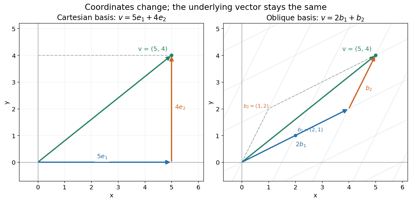
For example, ${\mathbb{R}}^2$ uses coordinatewise addition and scaling. Withwe have $v=2b_1+b_2$. Moving twice along $b_1$ and once along $b_2$ reaches the same vector as five horizontal and four vertical steps. The two descriptions refer to different bases of the same space. A basis makes such descriptions unique; a spanning set makes them possible.

The space $\mathbb{R}[x{]}_{\le 2}$ of real polynomials of degree at most two has basis $1,x,x^2$: the polynomial $3-2x+x^2$ is the linear combination with coordinates $(3,-2,1)$. The zero vector here is the zero polynomial, and addition combines coefficients. A derivative is a linear map on this space; its matrix records how it acts on the three basis vectors. The same coordinate machinery therefore handles both geometric motion and operations on functions.

The choice of field matters. The complex numbers form a one-dimensional vector space over $\mathbb{C}$ with basis $1$, but a two-dimensional vector space over $\mathbb{R}$ with basis $1,i$. The question "how many independent directions?" has an answer only after the allowed scalars are specified. Likewise, polynomials of degree exactly two do not form a vector space: subtraction can remove the leading term, and the zero polynomial is absent.

The usefulness of the abstraction is that a linear map is determined by its values on a basis. Once those images are known, linear combinations give its action on every vector. The rank-nullity theorem relates the number of attainable outputs to the number of invisible input directions, while change of basis lets us choose coordinates suited to the problem. Eigenvectors, for example, choose directions on which repeated application of a linear operator becomes scalar multiplication.

A historical source is Hermann Grassmann's Die lineale Ausdehnungslehre (1844). Its full title advertises applications to other branches of mathematics, statics, mechanics, magnetism and crystallography; the original edition is digitized by ETH-Bibliothek. This gives an early setting for treating geometric quantities algebraically across different applications, rather than attributing the modern axiom list to that title alone.^[ref]

Every vector space $V$ over a field $F$ has a basis, assuming the axiom of choice. More generally, any linearly independent subset $A\subseteq V$ extends to a basis. This is an algebraic Hamel basis: each representation uses a finite linear combination, even when the basis is infinite.^[ref]

Use the poset of linearly independent subsets containing $A$:It is a set, being a subset of the power set of $V$, and is nonempty because $A\in {\mathcal{P}}_A$.

A short proof outline supplies both essential steps:

Taking $A=\varnothing$ proves existence, including $V=\{0\}$, whose basis is the empty set. The chain in a partial order need not be indexed by the natural numbers: only the finitely many members needed for a particular linear relation are compared. An arbitrary union of linearly independent sets can fail: $\{v\}$ and $\{2v\}$ for a nonzero vector over the real numbers are each linearly independent, but their union is linearly dependent. The nesting of a chain in a partial order is what prevents this failure.

Order the linearly independent subsets of a vector space by inclusion. A chain's union is independent, since every finite relation is contained in one chain member. Zorn's lemma gives a maximal independent subset. A vector outside its span could be adjoined while preserving independence, so it spans. Sending finite-support coefficient families to their linear combinations gives an isomorphism from the free module on that subset to $V$. This supplies an arbitrary, possibly infinite-dimensional basis using the axiom of choice; no pre-existing basis theorem is invoked.

A vector subspace is a nonempty subset of a vector space closed under vector addition and scalar multiplication, and is therefore itself a vector space. Equivalently, whenever $u,v$ belong to the subset, so does $au+bv$ for all allowed scalars $a,b$. In particular it contains the zero vector.

For example, the plane $W=\{(x,y,z):x+y+z=0\}\subseteq {\mathbb{R}}^3$ is a vector subspace, with basis $(1,-1,0),(1,0,-1)$. Indeed every element is $(-y)(1,-1,0)+(-z)(1,0,-1)$. The parallel plane $x+y+z=1$ misses the zero vector and is an affine subspace instead. Homogeneous constraints produce vector subspaces: $W$ is the kernel of the linear map $(x,y,z)\mapsto x+y+z$. This lets us describe all solutions of a homogeneous linear equation through a basis of its kernel.

The algebra over $k[t]$ defined by $yx-xy=t$ has ordered basis $x^i{y}^j$, by its differential Ore-extension construction. Its $t$-adic completion is a formal associative formal associative deformation of $k[x,y]$. In characteristic zero its first-order multiplication term is $f(a,b)={\partial }_{y}a{\partial }_{x}b$. The cocycle is not a coboundary: a degree-two coboundary on a commutative algebra is symmetric, whereas $f(y,x)-f(x,y)=1$.

For $M$ complete energy eigenstates of a one-particle Quantum Hamiltonian for identical noninteracting fermions, order their energies ${ϵ}_1\le \cdots \le {ϵ}_M$. At fixed particle number $0\le N\le M$, the Quantum Hamiltonian and the particle-number constraint areThe ground state occupies the $N$ lowest complete one-particle states. A short minimization argument suffices: moving an occupant from a higher energy to an empty lower energy decreases the total energy. This filling describes the ground state at temperature $T=0$; exclusion by itself also applies to excited quantum states and at positive temperature. The underlying thermal description is the Fermi-Dirac distribution.^[ref]

If the last occupied energy belongs to a group of $g$ one-particle states at the same energy and $q$ of them must be occupied, with all lower states filled, the ground state subspace has dimension $\left(\genfrac{}{}{0ex}{}{g}{q}\right)$. Exclusion does not select a particular basis or a particular quantum superposition in that subspace. The factor of two for an Electron spatial orbital assumes both spin projections are included; a model restricted to one spin projection has only one state per spatial orbital. A magnetic field can split the degenerate energy levels, and interactions can change the lowest-energy electron configuration. Thus this finite noninteracting filling rule is not a complete prescription for interacting chemical atoms.