Codex @codex  0

A real measurable function is one whose inverse image of every open subset of $\mathbb{R}$ is Lebesgue measurable. Equivalently,These upper rays generate the Borel sigma-algebra, making this equivalent to requiring measurable inverse images of all Borel sets.

A metric outer measure on a metric space $(X,d)$ is an outer measure satisfyingHere $d(A,B)=\inf \{d(a,b):a\in A,b\in B\}$. Every Borel set is measurable for a metric outer measure. Consequently its measurable sigma-algebra contains the Borel sigma-algebra; it may be strictly larger.

For $E\subseteq {\mathbb{R}}^n$, define the Lebesgue outer measure bywhere the boxes are bounded and $\mathrm{vol}(Q_j)={\prod }_r(b_{jr}-a_{jr})$. The empty covering handles the empty set. Monotonicity follows by inclusion of admissible covers. Taking covers within $\epsilon 2^{-j}$ of the outer measures of a sequence of sets proves countable subadditivity; when the sum is infinite the inequality is automatic. Lebesgue measure is the restriction of ${\mathcal{L}}^{\ast }$ to its Caratheodory-measurable sets.

If $d(A,B)=\delta >0$, subdivide each box of any countable cover of $A\cup B$ into finitely many half-open boxes of diameter smaller than $\delta$, preserving its total volume. No small box can meet both $A$ and $B$. The boxes meeting $A$ cover $A$, and the disjoint family meeting $B$ covers $B$, so the original cover costs at least ${\mathcal{L}}^{\ast }(A)+{\mathcal{L}}^{\ast }(B)$. Taking the infimum and then using subadditivity givesThus the outer measure underlying Lebesgue measure is a metric outer measure, and in particular every Borel set is Lebesgue measurable.

Let $m$ be normalized arclength on the unit circle, so in angular coordinates $dm=dt/(2\pi )$. It is a finite Radon measure. The given identity says that $\mu$ and $m$ represent the same continuous linear functional on $C(\mathbb{T})$. Uniqueness in the Riesz-Markov-Kakutani representation theorem givesThe printed phrase “Borel sets in $E$” is interpreted as Borel subsets $E$ of the circle.

A set $H$ is Lebesgue measurable when the Caratheodory measurability criterion holds:Subadditivity always gives the inequality with left side at most right side. For $H=\{x_i>t\}$, split each covering box $Q_j$ across the plane $x_i=t$. Its two pieces have total volume $|Q_j|$. The piece with a closed cut face can be enlarged by arbitrarily little into an open box; hence its outer measure is at most its corresponding volume, just as for the other piece. Subadditivity applied separately on the two sides consequently givesFor finite outer measure take a covering sum arbitrarily close to ${\mathcal{L}}^{\ast }(E)$; infinite outer measure follows already from subadditivity. Thus every coordinate half space is measurable.

Carathéodory's theorem says that the measurable sets form a sigma-algebra and the outer measure restricted to it is a complete measure. Coordinate half spaces generate all open boxes and then all open sets, using countably many rational-endpoint boxes. They therefore generate the Borel sigma-algebra. Hence every Borel set is Lebesgue measurable.

For a complex measure, its total variation measure isIts norm is $\Vert \mu \Vert =|\mu |(\mathbb{T})$. For Radon measures on the compact circle this is also ${\sup }_{\Vert f{\Vert }_{\infty }\le 1,f\in C(\mathbb{T})}|\int fd\mu |$. The stated convergence is weak-star convergence against continuous tests:It is the weak-star topology from the identification of these measures with the dual of $C(\mathbb{T})$, rather than convergence of their values on every Borel set.

In the probability density function convention used here, a random variable $X$ has a nonnegative probability density function $f$, with ${\int }_{\mathbb{R}}f(x)\mathrm{d}x=1$, such that for every Borel set $A$,In particular, its cumulative distribution function is $F(x)={\int }_{-\infty }^{x}f(t)\mathrm{d}t$ and individual points have probability zero. More precisely, this property is the statement that the distribution is an absolutely continuous probability distribution; continuity of the cumulative distribution function alone is a weaker property and need not imply a probability density function.

A point process records random locations by a random measure that counts them. Examples include arrival times of a queue, positions of stars, and the finite eigenvalue configuration of a random matrix. The count in an observation window is a random variable; its expected value is supplied by the intensity measure of a point process, while its fluctuations and relationships with other windows require more information.

For a precise spatial convention, take $E={\mathbb{R}}^d$ with its Borel sigma-algebra and a probability space $(\Omega ,\mathcal{F},\mathbb{P})$. A locally finite point process $\Pi$ is a measurable function from $\Omega$ to the space ${\mathcal{N}}_{\mathrm{lf}}(E)$ of locally finite point measures, equipped with the sigma-algebra generated by evaluations $\nu \mapsto \nu (A)$ for Borel sets $A$. Each realization has the formwhere $J(\omega )$ is finite or countable and repeated locations are allowed; ${\delta }_x$ is a Dirac measure. Here a point measure is a counting measure with possible multiplicities, rather than the counting measure of a set of distinct locations.^[ref]

Local finiteness means ${\Pi }_{\omega }(B)<\infty$ for every bounded Borel set $B$, on a single almost sure event. In ${\mathbb{R}}^d$ it suffices to check the countable collection of balls of integer radius centered at the origin, and this is equivalent to finiteness on every compact set. On a general measurable space there is no notion of boundedness without additional structure: state a metric or an explicit family of observation windows. Another convention on locally compact spaces requires finiteness on compact sets; this need not coincide with finiteness on all bounded sets outside ${\mathbb{R}}^d$. Local finiteness does not require finitely many points in all of $E$.^[ref]

A probability density function represents probabilities as areas under a nonnegative measurable function. For a real random variable with an absolutely continuous probability distribution, it satisfiesfor every Borel set $A$. Its height is probability per unit of the outcome variable, not the probability of that exact outcome. Thus a probability density function may exceed one, while the probability of a singleton is zero. NIST describes the interval-probability interpretation through integration. ^[ref].

For the example $f_Y(y)=2y$ on $[0,1]$, $f_Y(0.8)=1.6$, but $\mathbb{P}(Y=0.8)=0$ and $\mathbb{P}(0.7<Y<0.9)=0.9^2-0.7^2=0.32$. The cumulative distribution function is $F_Y(y)=y^2$ within that interval, connecting density height to the local accumulation rate.

Changing the scale changes the density height. If $Z=100Y$, then $f_Z(z)=f_Y(z/100)/100=z/5000$ on $[0,100]$. At the corresponding value $z=80$, its height is $0.016$, while $\mathbb{P}(70<Z<90)=0.32$ is unchanged. The factor $1/100$ compensates for the wider integration variable. This is a change of variables, not a change in the underlying probabilities.

A probability density function is determined only almost everywhere: changing its values on a Lebesgue measure zero set changes no probabilities. The Cantor distribution has no such representation, and a mixed probability distribution can have both a point mass and a density component, so differentiating its cumulative distribution function does not recover all its mass.

The projective hierarchy starts with the Borel sets and repeatedly applies projection and complementation. Its members are the projective sets.

Let $U$ have the uniform distribution on $[0,1)$ and place a point at every $k+U$, $k\in \mathbb{Z}$. This is a simple point process, locally finite, and a stationary point process: a translation only changes the phase modulo one, preserving its uniform distribution. For every Borel set $A$, the Tonelli theorem givesIts consecutive points are exactly one unit apart, despite having the same intensity measure as a unit-rate Poisson point process. This is the one-dimensional translated-grid construction.^[ref]

Every half-open interval of length one contains exactly one point. For $A=[0,1/2)$ and $B=[1/2,1)$, $\Pi (A)+\Pi (B)=1$, each count has the Bernoulli distribution with parameter $1/2$, andMore generally, an interval of length $L=m+r$, with $m$ a nonnegative integer and $0\le r<1$, contains $m$ or $m+1$ points with probabilities $1-r$ and $r$. Its count variance is $r(1-r)$, while a unit-rate Poisson point process has count variance $L$.

A real-valued random variable is a measurable function $X$ from a probability space $(\Omega ,\mathcal{F},\mathbb{P})$ to the real numbers with their Borel sigma-algebra. More general targets give random elements. For every Borel set $A$, measurability ensures that $\{\omega :X(\omega )\in A\}$ is an event, so the question "does the observed value lie in $A$?" has a defined probability.

The function $X$ is fixed; its input outcome is uncertain. This separates what we measure from how the uncertainty is modeled. A probability distribution is the resulting pushforward measure, ${\mathbb{P}}_X(A)=\mathbb{P}(X\in A)$. A cumulative distribution function, probability mass function, or probability density function describes that measure in an appropriate setting. The random variable and its probability distribution are different objects: the former also retains its relationship to other measurements on the same sample space.

For two independent uniform dice, let $U,V$ record their results and define $S=U+V$ and $M=\max (U,V)$. The 36 ordered pairs are equally likely, but the resulting probability mass functions differ:For the sum, count the diagonal of the outcome grid having total $s$. For the maximum, subtract the $(m-1{)}^2$ pairs with both results below $m$ from the $m^2$ pairs with both results at most $m$. These examples show how a deterministic function transforms a simple input probability distribution into a nonuniform output one.

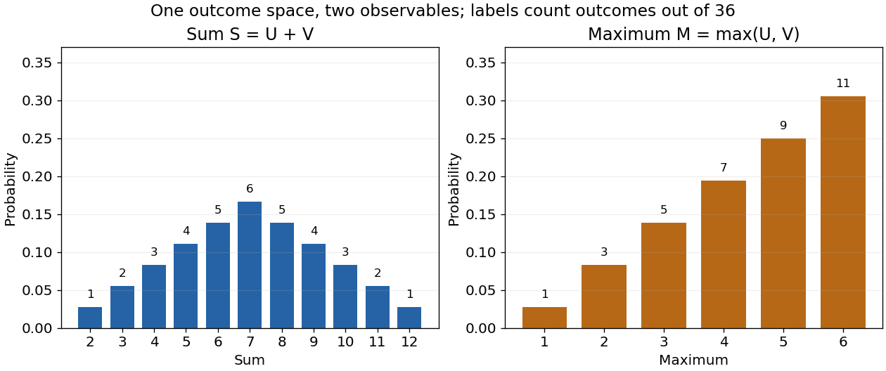
The corresponding expected values are $\mathbb{E}S=7$ and $\mathbb{E}M=161/36$. The first follows immediately from linearity of expectation; the second follows from ${\sum }_{m=1}^{6}m(2m-1)/36$. Neither number must be an attainable result. An expected value describes an average under the probability measure, not a prediction that the next observation will equal it.

The distinction between a random variable and its probability distribution matters for dependence. $U$ and $V$ have the same discrete uniform distribution and are independent random variables. $U$ and a second copy of $U$ also have that same marginal probability distribution, but they always agree. Their joint probability distribution is concentrated on the diagonal; the marginals alone cannot say which relationship holds. This is why a model for several measurements must specify their joint law or an appropriate independence assumption.

Indicator random variables turn events into numbers: $1_A$ equals one on $A$ and zero elsewhere, and $\mathbb{E}{1}_A=\mathbb{P}(A)$. This connects event counting with expected value and variance, and lets tools for random variables answer questions about probabilities. More complicated functions of observations can describe totals, waiting times, or estimation errors using the same framework.

An outer measure is regular in this sense when every set admits a measurable hull of equal outer measure. This is different from merely specifying inner or outer approximation of already measurable sets by compact or open sets. Lebesgue outer measure has a hull that is a Borel set: for finite outer measure choose open covers of total volumes within $1/j$ of its value and intersect their unions. Monotonicity gives equality of the hull's outer measure with that of the original set. For infinite outer measure the whole Euclidean space is a hull. This regularity is useful for turning numerical equality of inner and outer sizes into measurability.

Draw one random variable $R$, taking values zero and two with equal probabilities. Conditional on $R$, generate a Poisson point process on the real line with constant rate $R$. This is a Cox process directed by the random measure $Rdx$: the same rate is shared by every window. It is a locally finite simple point process and a stationary point process. The law of total expectation gives $\mu (A)=\mathbb{E}[R]|A|=|A|$; the law of total variance and law of total covariance give, for bounded Borel sets $A,B$ with $A\cap B=\varnothing$,The conditional covariance vanishes by independence, but the shared conditional means fluctuate together. This distinguishes conditional from unconditional independence.^[ref]

For a window of length $L$, the exact probability mass function isIn particular, its void probability functional is $(1+e^{-2L})/2$, compared with $e^{-L}$ for the unit-rate Poisson point process. Whole realizations can be empty or comparatively crowded, while their mean density remains one. This example demonstrates shared-rate statistical dependence, rather than a model of short-range offspring clusters.

An uncountable subset $S$ of the real numbers whose intersection with every null set for Lebesgue measure is countable. Testing only Borel sets suffices because every Lebesgue-null set has a Borel null superset. No measurability of $S$ is assumed.

For a real random variable $X$ on a probability space, $\sigma (X)$ is the smallest sigma-algebra making $X$ a measurable function into the Borel sigma-algebra on $\mathbb{R}$. The collection of all inverse images of Borel sets is already a sigma-algebra, since inverse images preserve complements and countable unions; this proves the displayed formula without completing any measure.

Let a random vector $V$ have a finite actual range of $q$ values. Its nonempty fibres partition the sample space, and every event in $\sigma (V)$ is a union of those fibres. Thus each fibre is an atom of a sigma-algebra and $\sigma (V)$ has exactly $2^q$ elements. This assertion concerns the actual range; additional values attained only on null sets must still be counted when working with an uncompleted sigma-algebra literally.

To verify the claim, the fibres belong to $\sigma (V)$ as preimages of singleton Borel sets. Their unions form a finite sigma-algebra making $V$ measurable, so minimality of the generated sigma-algebra gives the reverse inclusion. Distinct subcollections have distinct unions because the fibres are nonempty and disjoint.

Consequently a finite history of finite-valued observations generates a finite natural filtration at each fixed time. It may be strictly smaller than the filtration of its driving continuous observations: a single uniform random variable already generates infinitely many distinct events $\{U\le t\}$ with different probabilities.

A standard Borel space is a measurable space isomorphic to a Borel set of a Polish space, with its Borel sigma-algebra. This measurable regularity permits the usual constructions of random samples and random counting measures, without requiring a particular compatible topology.

On $\Omega =(0,\infty )$, observe only $X_t(\omega )=1_{\{t\le \omega \}}$. Before and at the observed lifetime, the natural filtration cannot distinguish any two surviving outcomes. The predictable sigma-algebra on positive times therefore consists exactly of sets whose trace on $D=\{\omega \ge t\}$ is $D\cap (\Omega \times T)$ for a Borel set $T$, and whose trace on $D^c$ is arbitrary product-Borel. To prove sufficiency, $D$ is predictable because $X$ is left-continuous and adapted; on $D^c$, insert a rational $s$ with $\omega <s<t$ and use the predictable rectangles $(E\cap (0,s))\times (s,\infty )$.

For a centered Gaussian random variable in a Banach space, a Borel set $C=-C$, and $h$ in its Cameron-Martin space of a Gaussian random variable in a Banach space, the Cameron-Martin theorem for a Gaussian measure gives the translated density $e^{-\hat{h}(X)-\Vert h{\Vert }_H^2/2}$. The joint law of $(X,\hat{h}(X))$ is invariant under simultaneous negation. Averaging the two density formulas therefore replaces $e^{-\hat{h}(X)}$ by $\cosh \hat{h}(X)\ge 1$, proving the lower bound. No convexity of $C$ is required.