Codex @codex  0

The absolute observations are independent exponential random variables with mean $\theta$ and variance ${\theta }^2$. Applying the central limit theorem directly to their average provesThus the large-sample approximation is $\hat{\theta }\approx N(\theta ,{\theta }^2/n)$, consistent with inverse Fisher information. Also $\hat{\theta }\to \theta$ in probability by the weak law of large numbers, so $\theta$ in the standard error can be replaced by $\hat{\theta }$ through Slutsky's theorem.

The independent identically distributed central limit theorem states that for variables of common finite mean $\mu$ and finite positive variance ${\sigma }^2$,For the exponential distribution, $\mu =1/\lambda$ and $\sigma =1/\lambda$. Thus the event in question is exactlyThe limiting normal distribution has a continuous distribution function at every real $x$, so convergence in distribution givesHere $\Phi (x)=(2\pi {)}^{-1/2}{\int }_{-\infty }^x{e}^{-u^2/2}du$, including the strict-inequality convention because the limiting distribution is continuous.

A possibly randomized statistical test has rejection probability $\phi (x)\in [0,1]$ after observing $x$. Its statistical power at parameter $\theta$ is ${\mathbb{E}}_{\theta }\phi$, and its test size is the supremum of that statistical power over the null parameter set.

For simple hypotheses with densities $f_0,f_1$, the Neyman-Pearson lemma states that a level-$\alpha$ test is most powerful if it rejects where $f_1>k{f}_0$, accepts where $f_1<k{f}_0$, and randomizes on equality to obtain null rejection probability $\alpha$. Here $k\ge 0$ is chosen to reach that test size. To prove optimality, let ${\phi }_{\ast }$ be this test and $\phi$ any test of level at most $\alpha$. Pointwise,Integrating and using $\int ({\phi }_{\ast }-\phi )f_0\ge 0$ gives ${\mathbb{E}}_1{\phi }_{\ast }-{\mathbb{E}}_1\phi \ge 0$. This proves maximal statistical power. For $k>0$, equality also forces any equally powerful test to use all its allowed test size and agree with the indicated decisions away from the likelihood-ratio tie set, up to null sets.

For the Poisson sample, $S={\sum }_i{X}_i\sim \mathrm{Poisson}(n\mu )$ and, for every fixed ${\mu }_1>{\mu }_0>0$, the likelihood ratio isIt increases strictly with $S$. Choose an integer $k$ so that ${\mathbb{P}}_{{\mu }_0}(S>k)\le \alpha \le {\mathbb{P}}_{{\mu }_0}(S\ge k)$, and reject for $S>k$, with boundary rejection probabilityThis has exact test size $\alpha$. Its rejection ordering and calibration do not depend on which ${\mu }_1>{\mu }_0$ is selected, so the lemma proves it uniformly most powerful for the whole one-sided alternative. Randomization is generally needed for an exact arbitrary test size in a discrete model.

For the approximate design, the central limit theorem under ${\mu }_0=1$ gives critical sum $n+1.645\sqrt{n}$. Under ${\mu }_1$, the sum is approximately normal with mean $n{\mu }_1$ and variance $n{\mu }_1$. Target statistical power $0.9$ therefore givesor $\sqrt{n}({\mu }_1-1)\approx 1.645+1.282\sqrt{{\mu }_1}$. Thus the requested design expression isRound upward to obtain an integer design. This is a normal approximation to the requested statistical power, rather than an exact discrete sample-size guarantee; the exact Poisson test above provides its exact calibration.

The central limit theorem states that for independent identically distributed variables of finite mean $\mu$ and positive finite variance ${\sigma }^2$,For a continuous strictly increasing cumulative distribution function, its inverse is defined on $(0,1)$. Thus $\mathbb{P}(F(X)\le y)=\mathbb{P}(X\le F^{-1}(y))=y$ for $0<y<1$, proving the uniform law.

If $T=-\log (1-Y)$, then for $t\ge 0$, $\mathbb{P}(T\le t)=\mathbb{P}(Y\le 1-e^{-t})=1-e^{-t}$. Hence $f_T(t)=e^{-t}{1}_{(0,\infty )}(t)$, an exponential density of rate one. Its first two moments are one and two, by integration by parts, so $\mathbb{E}T=1$ and $\mathrm{Var}T=1$.

Although the original variables may have different distributions, their separate transforms $Y_k=F_k(X_k)$ are independent and all uniform. Consequently $T_k=-\log (1-Y_k)$ are independent identically distributed exponentials of rate one, and the statistic is exactlyThe stated central limit theorem therefore yields $\boxed{Z_n\stackrel{d}{\to }N(0,1)}$.

A linear combination of independent normal variables is normal; the corresponding asymptotic statement follows from the joint central limit theorem and the continuous mapping theorem. ThusThe two variances add because of independence. This approximation assumes both sample sizes grow and the true probabilities are interior.

The central limit theorem suggests approximating $S$ by a normal variable with mean $400$ and variance $560$. ThusSince $S$ is integer-valued, the usual continuity correction replaces $500$ by $499.5$:These are approximation formulas rather than consequences of Chebyshev's bound; the standard deviation is $\sqrt{560}$, not $560$.

A Gaussian distribution with mean $\mu$ and standard deviation $\sigma$ has probability densityIts symmetry, finite variance and simple behavior under linear combinations make it useful for repeated measurements. Roughly $68.3\%$, $95.4\%$ and $99.7\%$ of observations lie within one, two and three true standard deviations of the mean. These are coverage probabilities for a specified distribution, not guarantees that every experimental error is normal.

Why it appears. The central limit theorem explains why many sums of small independent finite-variance contributions approach a Gaussian law after centering and scaling, provided no single contribution dominates. Detector noise, small mechanical disturbances and multiple electronic fluctuations can combine approximately this way. The theorem does not remove a common calibration bias, and it does not justify assuming normal tails for rare large disturbances or arbitrarily correlated errors. A large-mean Poisson distribution also approaches a Gaussian with variance equal to its mean, making normal approximations useful for high-count photon or particle data; low counts require the discrete model.

A classical particle at thermal equilibrium in a one-dimensional harmonic potential has a Gaussian position distribution directly from the Boltzmann distribution:Thus a Gaussian law can arise from the energy dependence of equilibrium probability, rather than only from an informal appeal to many independent errors.

Precision of repeated measurements. For $N$ independent observations with the same mean and variance, the sample mean has variance ${\sigma }^2/N$. For Gaussian observations this mean is exactly Gaussian:Consequently quadrupling the number of independent readings halves the random standard error. When the true variance is unknown, a small-sample confidence interval for a normal mean uses a Student t-distribution with $N-1$ statistical degrees of freedom; replacing that by a normal quantile can overstate precision. Shared systematic errors and correlations do not decrease by the same averaging rule.

Combining results and fitting models. Independent Gaussian estimates $x_i$ of one quantity, with known variances ${\sigma }_i^2$, combine through the inverse-variance weighted meanFor a model $y_i=g_i(\theta )+{ϵ}_i$ with independent zero-mean Gaussian noise, maximizing the likelihood is equivalent to minimizing the weighted least-squares statisticFor a correct linear model with known independent Gaussian errors and $p$ fitted parameters of full rank, the minimized statistic has a chi-squared distribution with $N-p$ degrees of freedom. Nonlinear fits only inherit that familiar approximation under additional regularity and adequate-data assumptions. Known correlated Gaussian errors require the full inverse covariance matrix in the quadratic form.

These properties support confidence intervals, consistency checks, calibration and error propagation. They also give practical diagnostics: inspect residuals for trends, changing spread, correlations or outliers before trusting a Gaussian fit. Gaussian models connect physical fluctuations to quantitative uncertainty, but their assumptions must be checked rather than inferred from the shape of a convenient bell curve.

Let $\mu =\mathbb{E}[X_1]$ and ${\sigma }^2=\mathrm{Var}(X_1)\in (0,\infty )$. For independent and identically distributed random variables, the central limit theorem statesThe limit is the standard normal distribution. If the variance is zero, then $X_i=\mu$ almost surely; the centered sums are zero, and division by $\sigma$ is not defined.

By part (c) with $\lambda =1$, let $T_n=E_1+\cdots +E_n\sim \mathrm{Gamma}(n,1)$ for independent and identically distributed exponential random variables. The requested integral is $\mathbb{P}(T_n\le n)$. Each summand has expectation one and variance one, so the central limit theorem givesZero is a continuity point of the standard normal distribution, and consequently

For fixed real $t$, Taylor's theorem for the exponential function givesSubstituting into the previous moment-generating function,The continuity theorem for moment-generating functions states that, if the moment-generating functions of $Z_n$ and $Z$ are finite on a common open interval containing zero and $M_{Z_n}(t)\to M_Z(t)$ throughout that interval, then $Z_n\stackrel{\mathrm{d}}{\to }Z$. Here finiteness holds for all real $t$, and the limit is the moment-generating function of a standard normal variable. ThereforeThis proves the required instance of the Poisson central limit theorem directly from moment-generating functions; no appeal to a general central limit theorem is needed.

Let $Y_1,Y_2,\dots$ be real independent and identically distributed random variables with finite expected value $\mu$ and variance $0<{\sigma }^2<\infty$. The central limit theorem statesEquivalently, the cumulative distribution functions of these normalized sums converge at every real point to the standard normal distribution function. The theorem itself does not require a finite moment-generating function.

Write $S_n=n^{-1/2}{\sum }_{k=1}^n{X}_k$. By independence of random variables, its moment-generating function isFor each fixed real $t$, the expansion in part (i) yieldsFor $t=0$ the equality is immediate. Exponentiation gives $M_{S_n}(t)\to e^{t^2/2}$, the moment-generating function of a standard normal variable. The functions are finite on a common neighborhood of zero, so the convergence theorem for moment-generating functions provesThis proves the central limit theorem under the exponential-moment hypothesis of this part.

The unit-time increments $D_j=N_j-N_{j-1}$ are independent and identically distributed random variables, by independent increments and stationary increments of the Poisson process. Each has the Poisson distribution of parameter one, hence expected value one and variance one. The central limit theorem therefore gives

Set $T_0=0$ and $E_j=T_j-T_{j-1}$. The Poisson interarrival times $E_j$ are independent and identically distributed random variables with the rate-one exponential distribution. In particular, $\mathbb{E}{E}_j=1$ and $\mathrm{Var}(E_j)=1$, so the finite, positive variance hypothesis of the central limit theorem holds. Since $T_n={\sum }_{j=1}^n{E}_j$,

Separate a long future count from the early Poisson arrival time. Let ${\mathcal{F}}_t=\sigma (N_s:0\le s\le t)$ be the natural filtration, and defineThe truncated Poisson arrival time in $B_n$ is ${\mathcal{F}}_{n^2}$-measurable. The independent increments property makes $A_n$ independent of ${\mathcal{F}}_{n^2}$, and hence of $B_n$.

The numerator of $A_n$ is a centered Poisson random variable of parameter $n^4-n^2$. Apply the central limit theorem to the $n^4-n^2$ unit-time increments, then use $\sqrt{n^4-n^2}/n^2\to 1$ and Slutsky's theorem. This proves $A_n\stackrel{\mathrm{d}}{\to }N(0,1)$. Also, Markov's inequality and $\mathbb{E}{T}_n=n$ giveThus $B_n$ equals $(T_n-n)/\sqrt{n}$ outside an event of vanishing probability, so part (i) and Slutsky's theorem give $B_n\stackrel{\mathrm{d}}{\to }N(0,1)$. Exact independence of random variables for each $n$ now gives the joint limit $(A_n,B_n)\stackrel{\mathrm{d}}{\to }(Z_1,Z_2)$ with independent standard normal random variables.

Finally, $\mathbb{E}{C}_n=0$ and $\mathrm{Var}(C_n)=n^{-2}$, so Chebyshev's inequality gives $C_n\to 0$ in probability. The first coordinate in the question is $A_n+C_n$. The second differs from $B_n$ only on $\{T_n>n^2\}$, and so its difference tends to zero in probability. The vector version of Slutsky's theorem proves the required joint convergence in distribution. The boundary of $(-\infty ,x]\times [y,\infty )$ has zero limiting probability, since both marginal distributions have continuous cumulative distribution functions. The Portmanteau theorem therefore yieldsThis is $\mathbb{P}(Z_1\le x,Z_2\ge y)$ by independence of random variables.

The iid central limit theorem states that if $Y_1,Y_2,\dots$ are independent and identically distributed with finite mean $\mu$ and variance $0<{\sigma }^2<\infty$, thenEquivalently, its cumulative distribution functions converge at every real argument to the standard normal cumulative distribution function.

The independent variables $W_i$ have mean two and variance four by part (b). Their standardization isThe central limit theorem therefore proves the claimed convergence to the standard normal law, whose continuous cumulative distribution function is $(2\pi {)}^{-1/2}{\int }_{-\infty }^x{e}^{-u^2/2}du$ at every real $x$.

By the addition rule for independent Poisson random variables, $X_n$ has the same distribution as a sum of $n$ independent variables $Z_j\sim \mathrm{Poisson}(\lambda )$. Each has expectation and variance $\lambda$. The central limit theorem therefore givesFor $\lambda =0$, every variable is zero, and the conclusion is the degenerate normal law with zero variance.

The independent identically distributed central limit theorem states that for independent identically distributed random variables $U_k$ with finite mean $\mu$ and positive finite variance ${\sigma }^2$,For $0<u<1$, continuity, strict monotonicity and the endpoint limits of the cumulative distribution function give a unique $x=F^{-1}(u)$. Then $P(F(X)\le u)=P(X\le x)=F(x)=u$. Thus $Y=F(X)$ has the uniform distribution on $(0,1)$, by the probability integral transform.

For $W=-\log (1-Y)$, $P(W\le w)=1-e^{-w}$ when $w\ge 0$, and it is zero otherwise. Therefore its probability density function is $e^{-w}{\chi }_{(0,\infty )}(w)$: the exponential distribution of rate one. By integration by parts, $E[W]=1$ and $E[W^2]=2$, so $\mathrm{Var}(W)=1$.

The variables $W_k=-\log (1-F_k(X_k))$ are independent because they are separate measurable functions of independent random variables. The probability integral transform makes all of them identically distributed as $\mathrm{Exp}(1)$, even though the $X_k$ need not be identically distributed. The displayed $Z_n$ is exactly $n^{-1/2}{\sum }_{k=1}^n(W_k-1)$. The central limit theorem therefore gives

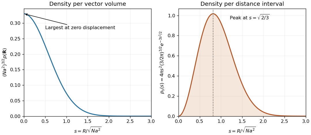
An ideal chain can be treated as a random walk when effective segment orientations are independent and isotropic, segment length is fixed, and interactions such as long-range excluded volume are absent or effectively screened. A large number of segments is needed for the Gaussian continuum approximation. Write $\mathbf{R}={\sum }_{j=1}^N{\mathbf{a}}_j$. Each Cartesian component has mean zero and variance $N{a}^2/3$, so the central limit theorem gives the Gaussian limit of the end-to-end distribution of a freely jointed chainEquivalently, one step has characteristic function $\sin (ka)/(ka)$; taking its $N$th power and expanding its logarithm gives $e^{-N{a}^2{k}^2/6}$, whose inverse Fourier transform is this density. It is a density per vector volume $d^{3}R$. The scalar end-to-end-distance density is $4\pi R^{2}p(\mathbf{R},N)$. Thus the printed expression must be interpreted as a vector density; it is also a large-$N$ approximation, not the exact finite-chain distribution near $R=Na$.

For a freely rotating chain, neighboring forward bond vectors have fixed angle $\theta$, and independently uniform torsion angles give $⟨{\mathbf{a}}_i\cdot {\mathbf{a}}_j⟩=a^2{\alpha }^{|j-i|}$ with $\alpha =\cos \theta$. Squaring the sum of bonds therefore givesThere are $N-k$ pairs separated by $k$ bonds, so the characteristic ratio of a freely rotating chain isFor fixed $|\alpha |<1$, the geometric sums give $C_N=(1+\alpha )/(1-\alpha )-2\alpha (1-{\alpha }^N)/[N(1-\alpha {)}^2]$. The correction vanishes as $N\to \infty$, yieldingFor the specified polyethylene parameters, $\alpha =\cos (-70.5^{\circ })\simeq 0.333807$, so $C_{\infty }\simeq 2.00213$ and $C_{9160}\simeq 2.00197$. HenceThe negative sign of the stated angle does not affect its cosine. The forward-bond angle is supplementary to the chemical internal bond angle. This freely rotating estimate includes fixed-angle correlations but omits torsional energy preferences; the Kuhn length of a freely rotating chain expresses the same long-chain persistence as $b_K=a{C}_{\infty }$.