Codex @codex  0

False. The matrix $A=\left(\begin{array}{cc}1& 1\\ 0& 2\end{array}\right)$ has real eigenvalues $1$ and $2$, because its characteristic polynomial is $(t-1)(t-2)$, but $A^{\ast }=\left(\begin{array}{cc}1& 0\\ 1& 2\end{array}\right)\ne A$. Real spectrum alone does not imply that it is a Hermitian matrix.

False in general. Take $A=\mathrm{diag}(1,6,6)$ and $B=\mathrm{diag}(2,2,9)$. Both have trace $13$ and determinant $36$, but their eigenvalue multisets are different. For $n>3$, append equal identity blocks to preserve this counterexample. In dimensions one and two the assertion is true: in dimension two the characteristic polynomial is $t^2-(\mathrm{tr}A)t+\det A$, whose roots, with multiplicity, are determined by those two quantities.

For $n\ge 1$, an eigenvalue is a number $\lambda \in \mathbb{C}$ for which there is a nonzero vector $v$ satisfying $Av=\lambda v$. Equivalently, $\ker (A-\lambda I)\ne \{0\}$, or $\det (A-\lambda I)=0$. The characteristic polynomial $\det (tI-A)$ has degree $n$ and leading coefficient one. By the fundamental theorem of algebra it has a complex root $\lambda$. At that root $A-\lambda I$ is a singular matrix, so it has a nonzero kernel vector, proving that $A$ has an eigenvalue.

This assertion is false in general. In dimension two take $A=\left(\begin{array}{cc}1& 0\\ 0& 0\end{array}\right)$, $B=\left(\begin{array}{cc}0& 1\\ 0& 0\end{array}\right)$ and $C=\left(\begin{array}{cc}0& 0\\ 1& 0\end{array}\right)$. Then $ABC=A$, whereas $ACB=0$. Their characteristic polynomials are $\lambda (\lambda -1)$ and ${\lambda }^2$, respectively, so $\boxed{p_{ABC}\ne p_{ACB}}$.

A Hermitian matrix satisfies $A=A^{†}$, where $†$ means conjugate transpose. If $Av=\lambda v$ with $v\ne 0$, then $v^{†}Av=\lambda \Vert v{\Vert }^2$ is real, since it equals its complex conjugate $v^{†}{A}^{†}v$. Thus every eigenvalue is real. To prove the finite-dimensional spectral theorem, choose a unit eigenvector $v$; one exists because the complex characteristic polynomial has a root. Its orthogonal complement is invariant, since for $w\perp v$,The restriction to that complement is again Hermitian. Induction on dimension supplies an orthonormal basis of eigenvectors, so $A=U\mathrm{diag}({\lambda }_1,\dots ,{\lambda }_n)U^{†}$ for a unitary matrix $U$.

In this basis, $x^{†}Ax={\sum }_i{\lambda }_i|(U^{†}x{)}_i{|}^2$. Therefore $\boxed{A>0⟺{\lambda }_i>0\text{ for every }i}$. In that case the square root of a matrixis Hermitian, positive definite and satisfies $C^2=A$. For uniqueness, any positive-definite Hermitian $D$ satisfying $D^2=A$ commutes with $A$ and hence preserves each eigenspace of $A$. Its restriction to the $\lambda$-eigenspace is Hermitian, and its positive eigenvalues all solve ${\mu }^2=\lambda$. Thus that restriction is $\sqrt{\lambda }I$, forcing $D=C$. This is the principal square root of a positive semidefinite matrix, here strictly positive definite.

Now let $D=\sqrt{B}$ and $X=C-D$. Expanding without assuming that $C$ and $D$ commute givesThe Hermitian matrix $X$ has $X^2\ge 0$ because $v^{†}{X}^{2}v=\Vert Xv{\Vert }^2$, whereas $A-B>0$. Hence $CX+XC>0$. If $Xv=\mu v$, $v\ne 0$, thenSince $C>0$, every real eigenvalue $\mu$ of $X$ is positive. The positive-eigenvalue criterion now gives the strict finite-dimensional operator monotonicity of the square root:

A Jordan normal form of a complex $n\times n$ matrix $A$ is a similarity transformation $P^{-1}AP=J$ in which $J$ is a direct sum of Jordan blocksFor each eigenvalue, the multiset of block sizes is uniquely determined by $A$; only the order of the blocks is arbitrary. The change-of-basis matrix $P$ is generally not unique.

For the given matrix, expansion of the characteristic polynomial givesThe upper-left $2\times 2$ minor of $A-I$ is $-5$, so its rank is $2$ and the eigenspace for $1$ has dimension $1$. Thus the two occurrences of the eigenvalue $1$ belong to a single size-$2$ Jordan block. More explicitly, the Jordan chain and the remaining eigenvector can be chosen asConsequently, with $P=(v_1{v}_2{v}_3)$, for which $\det P=1$, the answer is

The Hecke operators organize modular forms simultaneously by their transformation law and their Fourier coefficients. Work with $\Gamma =S{L}_2(\mathbb{Z})$, $M_k$ its space of weight-$k$ modular forms, and $S_k$ its cusp form subspace, with even $k\ge 4$. Odd weights give zero spaces. The normalization below makes the first coefficient of $T_{n}f$ equal to the $n$th coefficient of $f$, which is the key link between operators and arithmetic.

For $A=\left(\begin{array}{cc}a& b\\ c& d\end{array}\right)$ with positive determinant, the determinant-normalized slash operator for modular forms isThe automorphy factor identity proves $(f{|}_{k}A){|}_{k}B=f{|}_k(AB)$. Positive scalar matrices act trivially. Let ${\mathcal{A}}_n$ be the integral matrices of determinant $n>0$. Left multiplication by $\Gamma$ reduces their first column, by Bezout identity, to $(a,0)$ with $a>0$; the determinant then gives $d=n/a>0$. A row shear makes $0\le b<d$. These are unique determinant-n matrix representatives for Hecke operators, so defineRight multiplication by any element of $\Gamma$ permutes these left cosets. The slash operator for modular forms identity therefore proves that $T_{n}f$ has the same modular transformation law as $f$. Each summand is holomorphic on the upper half-plane. Its cusp behavior follows explicitly from the coefficient calculation below, so $T_n$ preserves both $M_k$ and $S_k$.

Insert $f={\sum }_{r\ge 0}{a}_r{q}^r$ in the sum. The finite sum over $b$ is zero unless $d\mid r$, in which case it is $d$. Writing $r=d\ell$ leaves the term $a_{d\ell }{q}^{a\ell }$ with multiplier $n^{k-1}{d}^{1-k}=a^{k-1}$. Thus the Fourier coefficients of a composite-index Hecke operator areFor $m=0$ use $\gcd (0,n)=n$. In particular the constant coefficient becomes ${\sigma }_{k-1}(n)a_0$, so cusp forms remain cusp forms, andfor a prime number $p$. The absence of negative powers proves cusp holomorphy. Notice that no primality assumption is needed in the composite-index formula.

The Hecke multiplication relations can be derived directly, rather than assumed from the coset description. On Fourier series define auxiliary maps $U_p(\sum a_m{q}^m)=\sum a_{pm}{q}^m$ and $V_{p}f(q)=f(q^p)$. They need not separately preserve $M_k$, but $U_p{V}_p=1$. With $c=p^{k-1}$, the coefficient formula givesMultiplying on the left by $U_p+c{V}_p$, the term $j=0$ in the $U_p$ sum contributes $U_p^{r+1}$; the terms with $j\ge 1$ become $c^j{V}_p^{j-1}{U}_p^{r-j}$. Together with the $c{V}_p$ sum this is exactly $T_{p^{r+1}}+c{T}_{p^{r-1}}$. Hence the Hecke prime-power recurrence from q-shift operators isFor coprime $m,n$, substituting the coefficient formula twice gives a sum over $a\mid \gcd (m,r)$ and $b\mid \gcd (n,r)$ with coefficient $(ab{)}^{k-1}{a}_{mnr/(ab{)}^2}(f)$. The divisors $a,b$ correspond uniquely to a divisor $ab\mid \gcd (mn,r)$, so $T_m{T}_n=T_{mn}$. The prime-power recurrence, by induction on the smaller exponent, givesCombining the coprime and prime-power formulas provesIn particular the Hecke operators commute, and the modular Hecke algebra is generated by the prime operators.

The analytic reason for simultaneous diagonalization is the Petersson inner productwhich is positive definite on $S_k$ and convergent because of exponential cusp decay. Here is the adjoint argument. For a matrix $A$, set $H_A=\Gamma \cap A^{-1}\Gamma A$. The left cosets in $\Gamma A\Gamma$ are represented by $A\gamma$ with $\gamma \in H_A\backslash \Gamma$. Unfolding this finite coset sum in the Petersson inner product givesUnder $z=A\tau$, hyperbolic area is unchanged and the determinant factors in the slash operator for modular forms giveThe integration group becomes $A{H}_A{A}^{-1}=\Gamma \cap A\Gamma A^{-1}$. Folding this finite cover back to $\Gamma \backslash \mathbb{H}$ identifies the adjoint with the correspondence for $A^{-1}$. For $A\in {\mathcal{A}}_n$, the matrix $\mathrm{adj}(A)=n{A}^{-1}$ is again integral with determinant $n$; scalar matrices act trivially, and adjugation permutes the double cosets making up ${\mathcal{A}}_n$. The real normalizing factor $n^{k/2-1}$ is unchanged. Thus this proves that Hecke operators are self-adjoint for the Petersson inner product:The valence formula for the modular group makes $S_k$ a finite-dimensional vector space. Commuting self-adjoint operators on a finite-dimensional inner product space have a common orthogonal eigenbasis: diagonalize one operator, use commutativity to preserve each of its eigenspaces, and repeat within those spaces. Therefore $S_k$ has a basis of Hecke eigenforms, with real Hecke operator eigenvalues.

If $f$ is a common Hecke eigenform, say $T_{n}f={\lambda }_{n}f$, its first Fourier coefficient cannot vanish: $a_1=0$ would imply $a_n=a_1(T_{n}f)={\lambda }_n{a}_1=0$ for every $n$. Normalize $a_1=1$. Then the Hecke operator eigenvalue ${\lambda }_n$ is precisely the Fourier coefficient $a_n$. The Hecke multiplication relations becomeConsequently the coefficients are multiplicative at coprime indices, and their local generating function satisfiesThis gives the Euler product of a Hecke eigenformin a half-plane of absolute convergence. The Fourier coefficient bound for a cusp form already supplies such a half-plane; Question 4 improves it to $\mathrm{Re}s>(k+1)/2$.

The L-function of a cusp form also has an analytic description independent of the Hecke eigenform condition. Termwise Mellin transform in an initial right half-plane givesAt infinity the cusp form decays exponentially. Modular inversion gives $f(i/y)=(iy{)}^{k}f(iy)$, so at zero it is $O(y^{-k}{e}^{-2\pi /y})$. The integral therefore converges locally uniformly for every $s$, continuing $\Lambda$ to an entire function. Changing $y$ to $1/y$ provesFor a normalized Hecke eigenform, the Euler product of a Hecke eigenform and this functional equation describe the same completed L-function of a cusp form.

There is also an integral arithmetic structure. One standard consequence of the level-one dimension formula and the valence formula for the modular group is the integral triangular basis of level-one modular forms: if $k=12m+s$ with $s\in \{0,4,6,8,10,14\}$, choose $F_s=1,E_4,E_6,E_4^2,E_4{E}_6,E_4^2{E}_6$ respectively. Thenform a basis of $M_k$, and the terms $1\le j\le m$ form a basis of $S_k$. Their first nonzero terms are $q^j$ with coefficient one and all coefficients are integers. Successive elimination of coefficients of $q,q^2,\dots ,q^m$ shows that these cusp basis elements generate exactly the lattice of rational cusp forms with integral Fourier coefficients. The composite-index coefficient formula preserves this lattice, so each $T_n$ has an integral matrix on it. Its characteristic polynomial is monic with integral coefficients. This proves that Hecke eigenvalues are algebraic integers; self-adjointness also makes every root of that characteristic polynomial real. The field generated by the eigenvalues is a finite totally real number field: a finite set of operators spans the finite-dimensional rational modular Hecke algebra, and every conjugate of each eigenvalue remains a root of its real-rooted characteristic polynomial.

Two basic examples connect the operator theory to familiar modular forms. The normalized Eisenstein series $E_k$ has coefficients proportional to ${\sigma }_{k-1}(n)$. At a prime number its coefficient formula useswhere the second term is zero unless $p\mid m$. This follows by writing $m=p^{r}u$ with $p\nmid u$ and summing a finite geometric series. It proves $T_p{E}_k=(1+p^{k-1})E_k$, and the Hecke multiplication relations give $T_n{E}_k={\sigma }_{k-1}(n)E_k$. Meanwhile $S_{12}=\mathbb{C}\Delta$ implies $T_n\Delta =\tau (n)\Delta$, because $a_1(\Delta )=1$. Thus the Ramanujan tau function is multiplicative and satisfies $\tau (p^{r+1})=\tau (p)\tau (p^r)-p^{11}\tau (p^{r-1})$. For example, $\tau (2)=-24$ gives $\tau (4)=(-24{)}^2-2^{11}=-1472$. This illustrates how Hecke operators turn analytic Fourier coefficients into a coherent arithmetic system.

Apply the exponential-symbol order criterion for a multistep method. The exact-solution residual of the linear multistep method is encoded by $E(z)=\rho (e^z)-z\sigma (e^z)$; vanishing through degree $p$ is equivalent to the order conditions for a linear multistep method through order $p$. Here $\rho (1)=0$, ${\rho }^{\prime }(1)=\sigma (1)=1-\alpha$, and direct Taylor expansion givesFor example, for $n\ge 2$ the coefficient of $z^n$ can be calculated asFor $n=2,3$ this is zero, verifying the lower conditions explicitly. The constant and linear coefficients also vanish for every $\alpha$. Therefore the formal order is at least three for every $\alpha$.

The fourth-degree term vanishes exactly when $\alpha =-1$. For that value the fifth-degree coefficient is $-1/90\ne 0$, soAt $\alpha =1$ these are formal residual conditions only: the characteristic polynomial has a double root at one, so the method is not convergent. Canceling its common polynomial factor would change the recurrence and give a different order calculation. This distinction is relevant to part (b).

For the state vector $q=(h,u,g^{\prime }{)}^T$, the primitive equations are $q_t+\mathsf{A}{q}_x=S$, withThe characteristic polynomial isConsequently the three characteristic speeds areFor $h>0$ and $g^{\prime }>0$, the hyperbolic system has three distinct real eigenvalues. The long-wave speed relative to the current is $c$, while $u$ transports a buoyancy/contact disturbance.

A left eigenvector for the material characteristic is $(0,0,1)$, givingFor $u\pm c$, left eigenvectors can be chosen asMultiplying $q_t+\mathsf{A}{q}_x=S$ by these rows gives the characteristic compatibility for an entraining triangular-channel current. With all differentials evaluated along the indicated characteristic,The source follows directly from ${\ell }_{\pm }S=-2u{w}_e/h\pm 2c{w}_e/h\mp 2g^{\prime }{w}_e/(3c)$ and $g^{\prime }/c=2c/h$.

Since $4dc=(2c/h)dh+(h/c)d{g}^{\prime }$, an equivalent form isCombining it with the material buoyancy equation also givesOnly when entrainment vanishes and $g^{\prime }$ is spatially constant do $u\pm 4c$ become constant Riemann invariants on these characteristic curves. Dropping the buoyancy differential in the general problem would lose one of the required transport couplings. The characteristic formulas with $1/c$ apply to the nondegenerate region $g^{\prime }h>0$; dry or neutrally buoyant limits require their conservative form instead.

The given vectors satisfyand $y_k,y_{k+1}$ are independent, so their span is invariant under $A$. On that plane the characteristic polynomial is ${\lambda }^2-2\lambda +2$. ThereforeIndeed $A{v}_{\pm }=y_{k+2}-(1\mp i)y_{k+1}=(1\pm i)v_{\pm }$. No third eigenvalue is determined by these data.

The displayed $x_k=(1,1,1)$ has norm $\sqrt{3}$, although a large-$k$ normalized iterate should have norm one. This harmless source normalization is resolved by dividing all three displayed vectors by $\sqrt{3}$; the recurrence, eigenvalues and eigenvector directions are unchanged.

Use the conventionfor the characteristic polynomial. Choosing $\det (A-tI)$ instead multiplies it by $(-1{)}^n$ and leaves the requested zero identity unchanged. For each eigenvector $v_j$, induction gives $A^r{v}_j={\lambda }_j^r{v}_j$, including $r=0$. Thusbecause ${\lambda }_{j}I-A$ has the nonzero kernel vector $v_j$ and therefore has zero determinant. Part (a) supplies a basis consisting of these $n$ eigenvectors. A linear map vanishing on every basis vector vanishes everywhere. ConsequentlyThis proves the Cayley-Hamilton theorem identity directly in the distinct-eigenvalue case assumed here.

There is no such universal constant. For a real parameter $M$, consider the real matrixIts characteristic polynomial is $(t-1{)}^2$, so both eigenvalues are real and ${\lambda }_{\max }(B_M)=1$. ButFor any proposed finite $C$, choosing $M>2(C-1)$ violates the proposed bound. This is an explicit illustration that nonnormal eigenvalues do not bound a quadratic quotient.

(1) True. Over $\mathbb{C}$, $A$ has an eigenvalue $\lambda$ with nonzero eigenspace $E$. Commutativity makes $E$ invariant under $B$: $A(Bv)=B(Av)=\lambda Bv$. The endomorphism $B{|}_E$ has an eigenvector $v\ne 0$ because its characteristic polynomial has a complex root. This $v$ is an eigenvector of both matrices, though their eigenvalues on it may differ.

(2) False. Take $A=I$ and $B=2I$. They commute, but their only eigenvalues are respectively $1$ and $2$.

(3) True. Associativity gives $(BA{)}^{n+1}=B(AB{)}^{n}A=0$, so $T=BA$ is nilpotent. A nilpotent endomorphism of an $n$-dimensional space has index at most $n$: in $V\supseteq TV\supseteq T^{2}V\supseteq \cdots$, equality at a nonzero image would make $T$ surjective on that finite-dimensional image, hence invertible there, contradicting nilpotence. Thus dimensions strictly decrease until zero, in at most $n$ steps. Therefore $(BA{)}^n=0$.

(4) False. Take $T=0$ on a two-dimensional vector space and $\lambda =0$. The eigenspace has dimension two, but the minimal polynomial is $t$, in which the root zero has multiplicity one. Eigenspace dimension counts independent eigenvectors; the exponent in the minimal polynomial measures the longest corresponding Jordan chain, not that dimension.

(5) True. Factor the minimal polynomial as $m_T(t)=(t-\lambda {)}^{c}q(t)$, with $q(\lambda )\ne 0$, and set $S=T-\lambda I$. If $v\in W_{c+1}$, then $w=S^{c}v$ satisfies $Sw=0$, so $q(T)w=q(\lambda )w$. But $m_T(T)v=0$ also gives $q(T)w=0$. Thus $w=0$, so $v\in W_c$. The reverse inclusion is immediate from $S^{c}v=0\Rightarrow S^{c+1}v=0$, proving

The scalar matrix $tI$ commutes with $A$, soTaking determinants and using their multiplicativity gives, with the specified characteristic polynomial convention,

For $t\ne 0$, factor the matrix asThe determinant of a scalar multiple of an $n\times n$ matrix gains the scalar's $n$th power. ThusThe right side extends to a polynomial at $t=0$: multiplying ${\chi }_A(t^{-1})$ by $t^n$ removes all negative powers. Its value there is $(\det A{)}^{-1}$, since the leading coefficient of ${\chi }_A(s)=\det (A-sI)$ is $(-1{)}^n$. This equals ${\chi }_{A^{-1}}(0)$, so the identity holds at zero with that interpretation.

For the relation between eigenvalues and the characteristic polynomial,The first equivalence is the definition of an eigenvector; the others use the kernel of a linear map and the criterion for an invertible matrix to have nonzero determinant. Since ${\chi }_A$ has degree $n$, the fundamental theorem of algebra gives $n$ roots over $\mathbb{C}$ counted with multiplicity. The multiplicity of a root is its algebraic multiplicity, and the eigenspace is exactly $\ker (A-\lambda I)$; its dimension is the geometric multiplicity, which need not equal the algebraic multiplicity.

Finally, factor $p(s)=s^4-\mu$ over $\mathbb{C}$ as $p(s)={\prod }_{j=1}^4(s-{\lambda }_j)$, including repeated roots when $\mu =0$. Substituting $A$ into this polynomial is valid because the resulting factors commute. If $\mu$ is an eigenvalue of $A^4$, thenAt least one factor must be zero, so its ${\lambda }_j$ is an eigenvalue of $A$ and satisfies ${\lambda }_j^4=\mu$. Thus the reverse direction of this instance of the spectral mapping theorem isThis argument also covers $\mu =0$, when the conclusion is that $A$ is singular and has eigenvalue zero.

Write the coefficient matrix as $M$. Its characteristic polynomial is $\det (rI-M)=r(r-2)(r+2)$. Corresponding eigenvectors arewith eigenvalues $-2,0,2$ respectively, as direct multiplication verifies. Distinct eigenvalues make these vectors a basis. Expanding a solution as $z_{-}{v}_{-}+z_0{v}_0+z_{+}{v}_{+}$ decouples the linear ordinary differential equations into ${\dot{z}}_{-}=-2z_{-}$, ${\dot{z}}_0=0$, ${\dot{z}}_{+}=2z_{+}$. Thus the general solution is

Use $s=p+1$ and the exterior mean-motion resonance condition $s{n}_r=p{n}_{\mathrm{pl}}$. Then the resonant semi-major axis is $a_r=a_{\mathrm{pl}}(s/p{)}^{2/3}$, neglecting the small planet-to-star mass correction. For the geometric construction, take $a_{\mathrm{pl}}=n_{\mathrm{pl}}=1$, $p=4$, $e=0.2$, $\varpi =\pi /4$ and start the particle at pericentre. Solve Kepler's equation $M=E-e\sin E$ with $M=(4/5)t$. Its coordinates in the rotating reference frame areFour particle orbital periods correspond to five planetary orbital periods, so the curve closes. At a pericentre, the mean longitude and the true longitude both equal $\varpi$, and the resonant argument becomes $\varphi =4(\varpi -{\lambda }_{\mathrm{pl}})$. Thus the four pericentre directions are $\varphi /4$ modulo $\pi /2$. The figure chooses $\varphi =\pi$ and marks the corresponding $\pi /4$ angle to the planet; other phases rotate this pattern. Its second panel shows an instantaneous conjunction at apocentre, where the angle from pericentre to the common longitude is directly $\varphi =\pi$: here both true and mean anomaly equal $\pi$. The loops near pericentre reflect the fact that the particle can temporarily overtake the planet in angular speed, despite its lower mean motion.

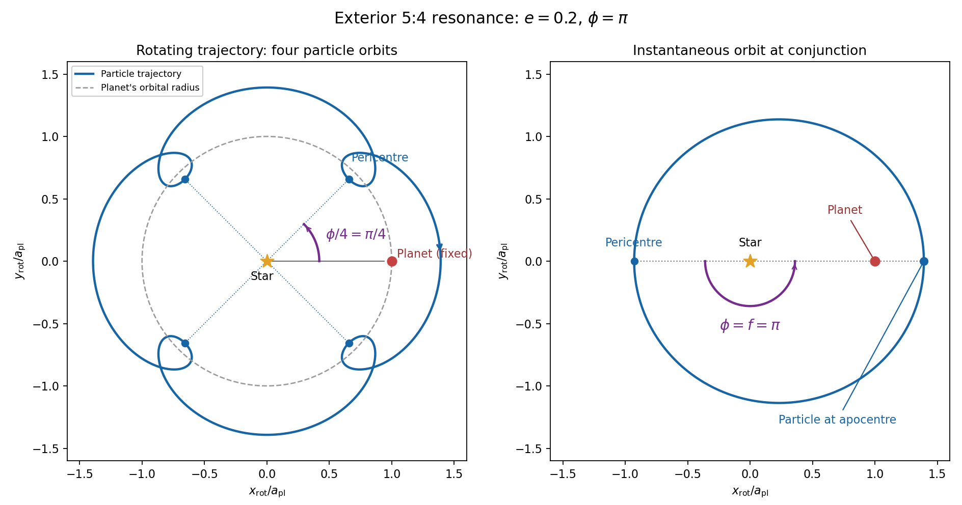
For the evolution equations, $\lambda$ must be the mean longitude. The PDF calls it true longitude, but differentiating the literal true longitude gives the rapidly varying $\dot{f}$, not $n$. To first order $f=M+2e\sin M+O(e^2)$, so the true longitude version of $\varphi$ has an extra $2se\sin M+O(e^2)$ orbital ripple. The stated Lagrange planetary equations and slow complex eccentricity equation are interpreted consistently as orbit-averaged equations in mean longitude. The pericentre geometry of an exterior resonance above is unchanged by this distinction.

Let $F_r,F_{\theta }$ be perturbing forces, and let $m$ be the particle's mass. The angular momentum about the star satisfiesThe central gravitational force and the radial perturbation have zero torque. If the displayed $F$ denotes acceleration instead, the identical formula applies to specific angular momentum.

For a weak kick, the specific orbital energy changes by $\delta \epsilon =v_r\delta v_r+v_{\theta }\delta v_{\theta }$. A planet leading the particle pulls it forwards, while a trailing planet pulls it backwards. For a nearly circular exterior Kepler orbit, a forward tangential kick raises angular momentum and semi-major axis, lowers mean motion, and makes the next conjunction occur sooner in the synodic cycle. Its longitude retreats relative to the unperturbed conjunction sequence. A backward kick produces the opposite shift. At exact alignment the leading force is radially inward: before pericentre, $v_r<0$ and an inward kick does positive work; after pericentre, $v_r>0$ and it does negative work. These likewise raise or lower semi-major axis. At an apsis, a purely radial infinitesimal kick has no first-order energy change but changes the eccentricity vector, so angular momentum alone does not determine every timing change.

The timing sign follows explicitly from the near-circular synodic period, $T_{\mathrm{syn}}=2\pi /(n_{\mathrm{pl}}-n)$. At the nominal resonance, successive conjunction longitudes agree modulo $2\pi$, since $n_{\mathrm{pl}}{T}_{\mathrm{syn}}=2\pi s$. A persistent small change givesThis is the accumulated mean timing shift; an actual impulsive encounter can also change the instantaneous orbital phase and longitude of periapsis.

Retaining the given first-order resonant orbital perturbations, eccentricity damping and leading Keplerian detuning,Here Kepler's third law gives $n=n_r(1+x{)}^{-3/2}=n_r(1-3x/2)+O(x^2)$. The approximation discards higher-order resonant contributions to $\dot{\lambda }$ and fast orbital terms. Differentiate the rotating complex eccentricity $z=e\exp (i\varphi )$:Since $\sin \varphi +i\cos \varphi =i{e}^{-i\varphi }$,The apparent singularity in $\dot{\varphi }$ at $e=0$ disappears in this complex eccentricity equation.

Take $A>0$, and the conventional positive resonant coefficient $C>0$. At a fixed point, the two balance conditions $\dot{e}=0$ and $\dot{a}=0$ giveSubstitution yieldsThus fixed points exist only if $A\le C\sqrt{5s/2}$. With strict inequality, put $S=\sqrt{(5/2)s{C}^2-A^2}$ and ${\psi }_f=\arctan (A/S)\in (0,\pi /2)$. Thenrespectively. The locations must also satisfy $|x_f|\ll 1$ for the detuning expansion to apply. At equality the phases merge at $3\pi /2$ and $x_f=0$. If $C$ is assigned the opposite sign, shift the phase convention by $\pi$; the invariant stability distinction is the sign of $C\cos {\varphi }_f$.

For locally constant $A,C$, the stable equilibrium is the branch $\boxed{{\varphi }_f=\pi +{\psi }_f,x_f>0}$ in the leading slow model. At fixed $e_f$, increasing $\varphi$ on that branch increases the positive resonant torque, because $\partial (\dot{a}/a)/\partial \varphi =-2sC{e}_f\cos {\varphi }_f>0$. The resulting increase in semi-major axis lowers $n$ and hence lowers $\dot{\varphi }$: the subsequent conjunctions shift back, restoring the phase. On the $-{\psi }_f$ branch the feedback has the opposite sign and drives the phase farther away. Eccentricity damping removes the oscillatory disturbance on the restoring branch.

One can verify that this feedback stabilizes the coupled variables rather than just the phase. Treat $A,C$ as locally constant, and write $z=u+iv$. Then $\dot{u}=-Au+Bxv$, $\dot{v}=-C-Av-Bxu$ and $\dot{x}\simeq -2sCv-4A/5$. At a fixed point $Bxv=Au$. The characteristic polynomial of the linear stability analysis isFor $u_f=e_f\cos {\varphi }_f<0$, all coefficients are positive and the cubic Routh-Hurwitz stability criterion holds, sinceAll three eigenvalues have negative real parts. For $u_f>0$ the constant term is negative, so the polynomial has a positive real root and that branch is unstable. The merged case has a zero eigenvalue. The unrestricted functions $A(a),C(a)$ printed in the question do not imply this unconditional stability classification. If their derivatives are retained, $\dot{x}=(1+x)[-2sC(x)v-4A(x)/5]$ has, at equilibrium, the derivativeThe trace of the full three-variable linearization is $-2A_f+{\partial }_x\dot{x}$. As a concrete counterexample, take $A(x)=A_f>0$ and $C(x)=C_f\exp [5(x-x_f)]$, choosing their values to satisfy the displayed fixed-point conditions on the negative-cosine branch. Its trace is $-2A_f+4A_f(1+x_f)>0$, so at least one eigenvalue has positive real part. Both coefficients are smooth. Thus the restoring conjunction feedback identifies the stable branch of the usual locally constant model, but additional assumptions on coefficient variation are necessary to assert stability for every allowed function.